Lab 1 – Introduction to R
Philipp Broniecki and Lucas Leemann – Machine Learning 1K
R Introduction (based on Leemann and Mykhaylov, PUBLG100)
Let’s get acquainted with R.
Take a look at R Studio. See the 4 windows:
- Upper-Left : R-script.
- Lower-Left : Console.
- Upper-Right : Environment (data, variables, …)
- Lower-Right : Plots, help file, packages etc.
We begin by walking through the steps for creating and saving an R script.
- Create a new R script and save it as lab1.R to your
StatisticalLearningdirectory. - Now type the following commands in the new file you just created:
# check working directory
getwd()
## [1] "C:/Users/phili/Documents/ML2017.io"Save your script, and re-open it to make sure your changes are still there. Then check your workspace.
# check workspace
ls()
# delete variable 'a' from workspace
rm(a)
# delete everything from workspace
rm( list = ls() )

# to clear console window press Crtl+l on Win or Command+l on Mac
Creating and manipulating variables, vectors, data frames
# Create a numeric and a character variable
a <- 5
typeof(a) # a is a numeric variable
## [1] "double"a## [1] 5b <- "Yay stats class"
typeof(b) # b is a string variable## [1] "character"b## [1] "Yay stats class"# Create a vector
my.vector <- c(10,7,99,34,0,5) # a vector
my.vector## [1] 10 7 99 34 0 5length(my.vector) # how many elements?## [1] 6# subsetting
my.vector[1] # 1st vector element## [1] 10my.vector[-1] # all elements but the 1st## [1] 7 99 34 0 5my.vector[2:4] # the 2nd to the 4th elements## [1] 7 99 34my.vector[c(2,5)] # 2nd and 5th element## [1] 7 0my.vector[length(my.vector)] # the last element## [1] 5# calculating in R
# element-wise operations
my.vector + 2 ## [1] 12 9 101 36 2 7my.vector * 2## [1] 20 14 198 68 0 10my.vector / 2## [1] 5.0 3.5 49.5 17.0 0.0 2.5my.vector ^2## [1] 100 49 9801 1156 0 25sqrt(my.vector)## [1] 3.162278 2.645751 9.949874 5.830952 0.000000 2.236068log(my.vector)## [1] 2.302585 1.945910 4.595120 3.526361 -Inf 1.609438Use the ? to get help on R functions. E.g. ?rep will open the help for the rep() function.
# creating longer vectors and sequences
na.vector <- rep(NA, 10)
na.vector
## [1] NA NA NA NA NA NA NA NA NA NAid.var <- seq(from = 1, to = length(na.vector), by = 1)
# combine vectors to data frame
my.df <- data.frame(id.var, na.vector)
my.df## id.var na.vector
## 1 1 NA
## 2 2 NA
## 3 3 NA
## 4 4 NA
## 5 5 NA
## 6 6 NA
## 7 7 NA
## 8 8 NA
## 9 9 NA
## 10 10 NA# create a matrix
my.matrix1 <- matrix(data = c(1,2,30,40,500,600), nrow = 3, ncol = 2, byrow = FALSE,
dimnames = NULL)
my.matrix1## [,1] [,2]
## [1,] 1 40
## [2,] 2 500
## [3,] 30 600# subsetting a matrix
my.matrix1[1,2] # element in row 1 and column 2## [1] 40my.matrix1[2,1] # element in row 2 and column 1## [1] 2my.matrix1[,1] # 1st column only## [1] 1 2 30my.matrix1[1:2,] # rows 1 to 2## [,1] [,2]
## [1,] 1 40
## [2,] 2 500my.matrix1[c(1,3),] # rows 1 and 3 ## [,1] [,2]
## [1,] 1 40
## [2,] 30 600Download the foreigners data set here. Copy it to your working directory and then load the data set using the load() function.
# load, inspect, and manipulate data set
load("./data/BSAS_manip.RData")
# variable names
names(data2)
## [1] "IMMBRIT" "over.estimate" "RSex" "RAge"
## [5] "Househld" "Cons" "Lab" "SNP"
## [9] "Ukip" "BNP" "GP" "party.other"
## [13] "paper" "WWWhourspW" "religious" "employMonths"
## [17] "urban" "health.good" "HHInc"# summary stats of all variables
summary(data2)## IMMBRIT over.estimate RSex RAge
## Min. : 0.00 Min. :0.0000 Min. :1.000 Min. :17.00
## 1st Qu.: 10.00 1st Qu.:0.0000 1st Qu.:1.000 1st Qu.:36.00
## Median : 25.00 Median :1.0000 Median :2.000 Median :49.00
## Mean : 29.03 Mean :0.7235 Mean :1.544 Mean :49.75
## 3rd Qu.: 40.00 3rd Qu.:1.0000 3rd Qu.:2.000 3rd Qu.:62.00
## Max. :100.00 Max. :1.0000 Max. :2.000 Max. :99.00
## Househld Cons Lab SNP
## Min. :1.000 Min. :0.0000 Min. :0.0000 Min. :0.00000
## 1st Qu.:1.000 1st Qu.:0.0000 1st Qu.:0.0000 1st Qu.:0.00000
## Median :2.000 Median :0.0000 Median :0.0000 Median :0.00000
## Mean :2.392 Mean :0.2707 Mean :0.2669 Mean :0.01525
## 3rd Qu.:3.000 3rd Qu.:1.0000 3rd Qu.:1.0000 3rd Qu.:0.00000
## Max. :8.000 Max. :1.0000 Max. :1.0000 Max. :1.00000
## Ukip BNP GP party.other
## Min. :0.00000 Min. :0.00000 Min. :0.00000 Min. :0.0000
## 1st Qu.:0.00000 1st Qu.:0.00000 1st Qu.:0.00000 1st Qu.:0.0000
## Median :0.00000 Median :0.00000 Median :0.00000 Median :0.0000
## Mean :0.02955 Mean :0.03051 Mean :0.02193 Mean :0.3651
## 3rd Qu.:0.00000 3rd Qu.:0.00000 3rd Qu.:0.00000 3rd Qu.:1.0000
## Max. :1.00000 Max. :1.00000 Max. :1.00000 Max. :1.0000
## paper WWWhourspW religious employMonths
## Min. :0.0000 Min. : 0.000 Min. :0.0000 Min. : 1.00
## 1st Qu.:0.0000 1st Qu.: 0.000 1st Qu.:0.0000 1st Qu.: 72.00
## Median :0.0000 Median : 2.000 Median :0.0000 Median : 72.00
## Mean :0.4538 Mean : 5.251 Mean :0.4929 Mean : 86.56
## 3rd Qu.:1.0000 3rd Qu.: 7.000 3rd Qu.:1.0000 3rd Qu.: 72.00
## Max. :1.0000 Max. :100.000 Max. :1.0000 Max. :600.00
## urban health.good HHInc
## Min. :1.000 Min. :0.000 Min. : 1.000
## 1st Qu.:2.000 1st Qu.:2.000 1st Qu.: 6.000
## Median :3.000 Median :2.000 Median : 9.000
## Mean :2.568 Mean :2.044 Mean : 9.586
## 3rd Qu.:3.000 3rd Qu.:3.000 3rd Qu.:13.000
## Max. :4.000 Max. :3.000 Max. :17.000# external excel-style explorer
#fix(data2)
# variable types in data frame
str(data2)## 'data.frame': 1049 obs. of 19 variables:
## $ IMMBRIT : num 1 50 50 15 20 30 60 7 30 2 ...
## $ over.estimate: num 0 1 1 1 1 1 1 0 1 0 ...
## $ RSex : num 1 2 2 2 2 1 2 1 1 1 ...
## $ RAge : num 50 18 60 77 67 30 56 49 40 61 ...
## $ Househld : num 2 3 1 2 1 4 2 1 4 3 ...
## $ Cons : num 0 0 0 0 0 0 0 0 0 1 ...
## $ Lab : num 1 0 0 0 0 0 0 0 0 0 ...
## $ SNP : num 0 0 0 0 0 0 1 0 1 0 ...
## $ Ukip : num 0 0 0 0 0 0 0 0 0 0 ...
## $ BNP : num 0 0 0 0 0 0 0 0 0 0 ...
## $ GP : num 0 0 0 0 0 0 0 0 0 0 ...
## $ party.other : num 0 1 1 1 1 1 0 1 0 0 ...
## $ paper : num 0 0 0 1 0 1 0 1 0 1 ...
## $ WWWhourspW : num 1 4 1 2 1 14 5 8 3 0 ...
## $ religious : num 0 0 0 1 1 0 1 0 1 1 ...
## $ employMonths : num 72 72 456 72 72 72 180 156 264 72 ...
## $ urban : num 4 4 3 1 3 1 1 4 2 1 ...
## $ health.good : num 1 2 3 3 3 2 2 2 2 3 ...
## $ HHInc : num 13 3 9 8 9 9 13 14 11 8 ...# indexing in data sets
# first 5 rows and first 4 columns (similar to matrix indexing)
data2[1:5, 1:4] ## IMMBRIT over.estimate RSex RAge
## 1 1 0 1 50
## 2 50 1 2 18
## 3 50 1 2 60
## 4 15 1 2 77
## 5 20 1 2 67# indexing with names using the $-sign
data2$RSex[1:5]## [1] 1 2 2 2 2# indexing with names using square brackets
data2[1:6, c("RAge", "WWWhourspW")]## RAge WWWhourspW
## 1 50 1
## 2 18 4
## 3 60 1
## 4 77 2
## 5 67 1
## 6 30 14# dimension of a data set
dim(data2)## [1] 1049 19# number of rows
nrow(data2)## [1] 1049# number of columns
ncol(data2)## [1] 19# delete a variable
data2$SNP <- NULL
# rename a variable
names(data2)[ names(data2) == "RAge" ] <- "age"
names(data2)## [1] "IMMBRIT" "over.estimate" "RSex" "age"
## [5] "Househld" "Cons" "Lab" "Ukip"
## [9] "BNP" "GP" "party.other" "paper"
## [13] "WWWhourspW" "religious" "employMonths" "urban"
## [17] "health.good" "HHInc"# creating a new (dummy) variable
data2$old <- ifelse( data2$age > 30, yes = 1, no = 0)
# frequency table of new variable
table(data2$old)##
## 0 1
## 176 873# create subesets
df.cons <- data2[ data2$Cons == 1 , ]
df.not_cons <- data2[ data2$Cons != 1, ]
# pick observations randomly
#?sample
pick <- sample(nrow(data2), size = as.integer(.33 * nrow(data2)), replace = FALSE)
df2 <- data2[ pick, ]
df3 <- data2[ -pick, ]Plotting
# scaterplot
plot(WWWhourspW ~ age, data = data2,
     main = "scatterplot")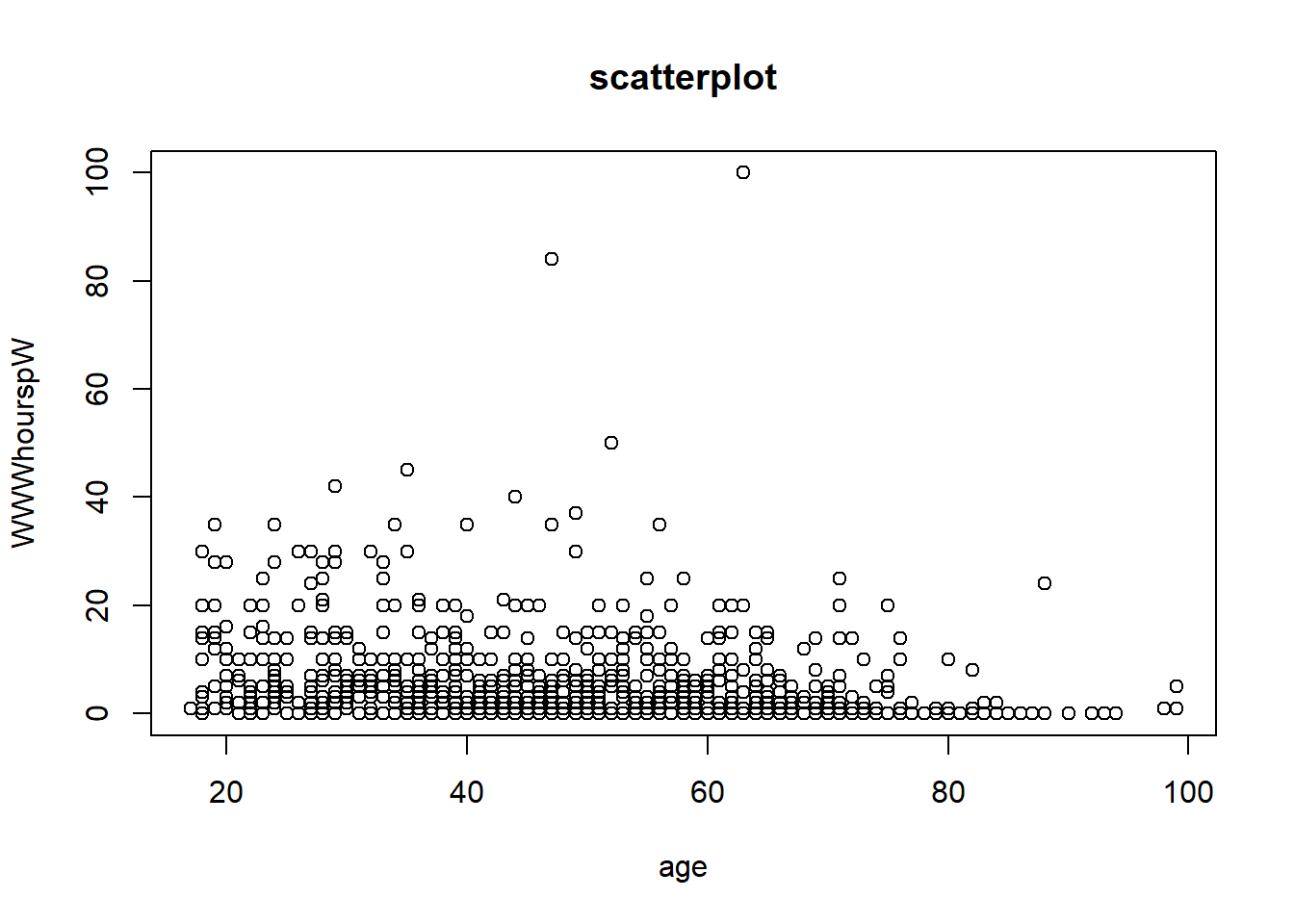
# boxplot
plot(HHInc ~ as.factor(Ukip), data = data2,
     main = "boxplot",
     xlab = "Ukip party affiliation",
     ylab = "income",
     frame.plot = FALSE)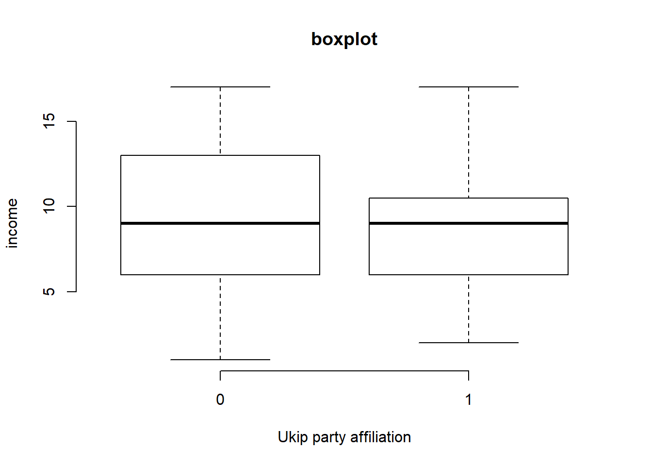
# density
plot( density(data2$employMonths), bty = "n", main = "density plot")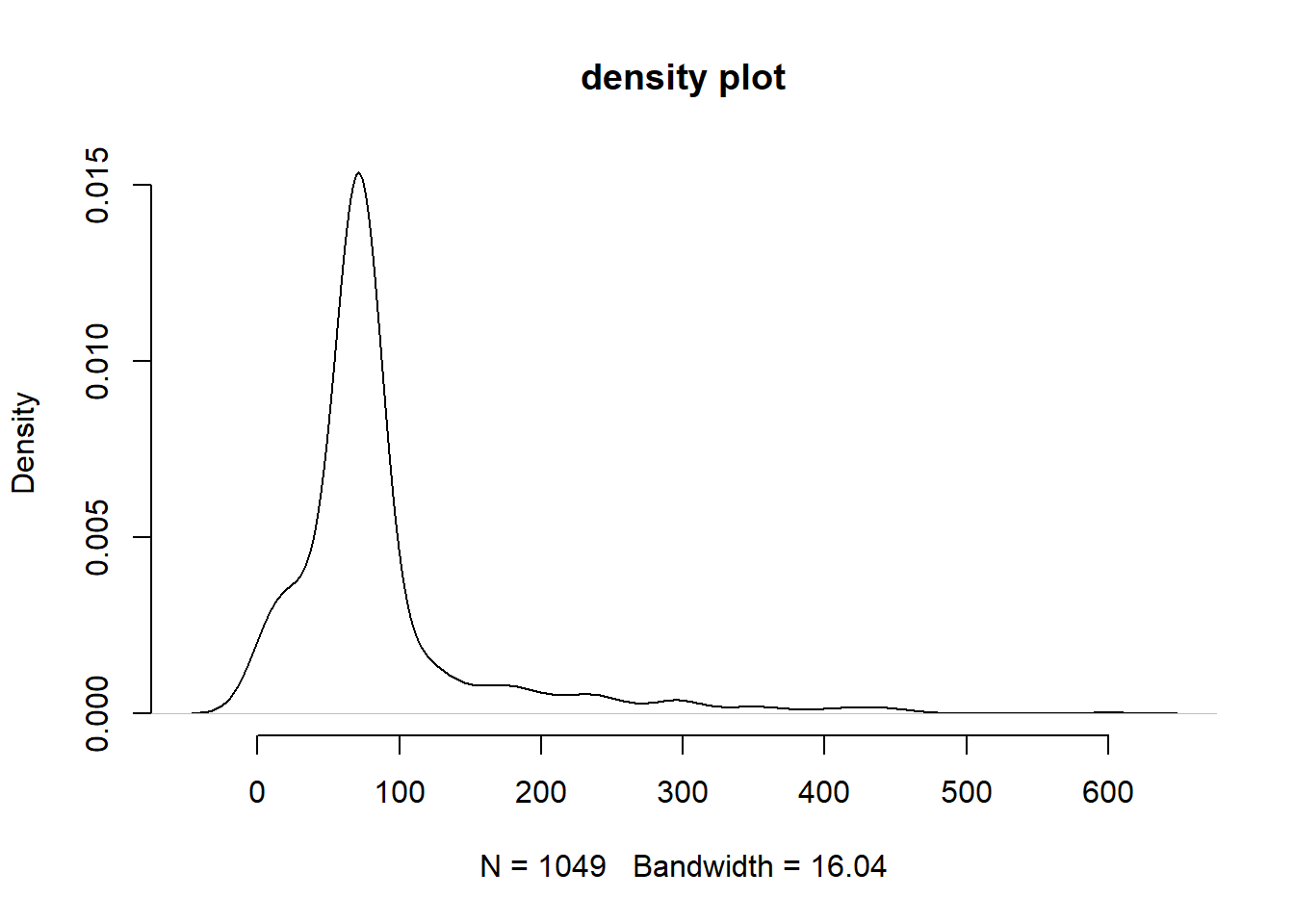
# histogram
hist( data2$employMonths, main = "histogram")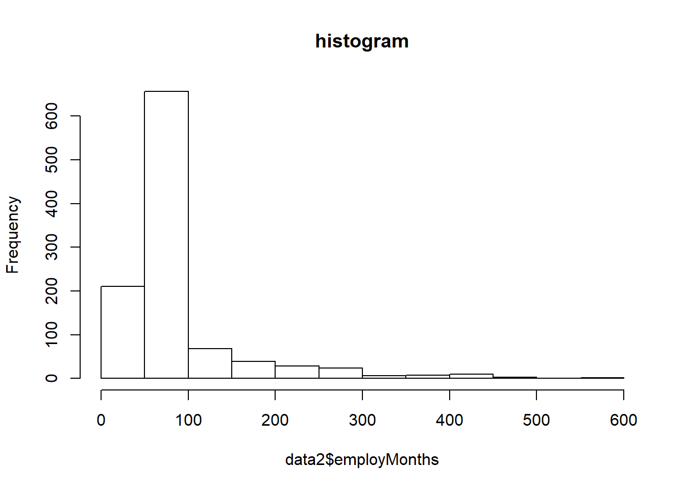
Download a useful cheat-sheet for R if you are not already familiar with the essentials of R. https://www.rstudio.com/wp-content/uploads/2016/06/r-cheat-sheet.pdf
Exercises 1
- Create a new file called “assignment1.R” in your
StatisticalLearningfolder and write all the solutions in it. - Clear the workspace and set the working directory to your
StatisticalLearningfolder. - Load the High School and Beyond dataset. Remember to load any necessary packages.
- Calculate the final score for each student by averaging the
read,write,math,science, andsocstscores and save it in a column calledfinal_score. - Calculate the mean, median and mode for the
final_score. - Create a factor variable called
school_typefromschtypusing the following codes:- 1 = Public schools
- 2 = Private schools
- How many students are from private schools and how many are from public schools?
- Calculate the variance and standard deviation for
final_scorefrom each school type. - Find out the ID of the students with the highest and lowest
final_scorefrom each school type. - Find out the 20th, 40th, 60th and 80th percentiles of
final_score. - Create box plot for
final_scoregrouped by theschool_typefactor variable to show the difference betweenfinal_scoreat public schools vs. private schools.
Packages
What are packages and why should I care?
Packages are bundled pieces of software that extend the functionality of R far beyond what’s available when you install R for the first time. Just as smartphone “apps” add new features or make existing features easier to use, packages add new functionality or provide convenient functions for tasks that otherwise would be cumbersome to do using base R packages. Some R packages are designed to carry out very specific tasks while others are aimed at offering a general purpose set of functions. We will get a chance to work with both specific and generic type of packages over the next several days.
A small number of core packages come pre-installed with R but thousands of extremely useful packages are available for download with just a few keystrokes within R. The strength of R comes not just from the language itself but from the vast array of packages that you can download at no cost.
Installing Packages
Recall from earlier that we used the read.csv() function to read a file in Comma Separated Values (CSV) format. While CSV is an extremely popular format, the dataset we’re using in this seminar is only available in Microsoft Excel format. In order to load this dataset we need a package called readxl.
We will install the readxl package with the install.packages() function. The install.packages() function downloads the package from a central repository so make sure you’ve internet access before attempting to install it.
install.packages("readxl")
Watch out for errors and warning messages when installing or loading packages.
Removing Packages
On rare occasions, you might have to remove a package from R. Although we will not demonstrate removing packages in this seminar, it is worth noting that the remove.packages() function can be used to remove a package if necessary.
Using Packages
Once a package is installed, it must be loaded in R using the library() function. Let’s load the readxl package so we can use the functions it provides for reading a file an Excel file. The library() function takes the name of the package as an argument and makes the functionality from that package available to us in R.
library(readxl)## Warning: package 'readxl' was built under R version 3.4.1Now that the readxl package is loaded, we can load our dataset. In this seminar, we’re using a small subset of High School and Beyond survey conducted by the National Center of Education Statistics in the U.S. Our dataset includes observations from 200 students with variables including each student’s race, gender, socioeconomic status, school type, and scores in reading, writing, math, science and social studies.
First, we need to download the dataset and save it to our StatisticalLearning folder. If you haven’t set your working directory yet, make sure to follow the Getting Started instructions from the top of this page.
Download ‘High School and Beyond’ Dataset
Next we load the dataset using the read_excel() function from the readxl package.
# make sure you've downloaded the dataset from http://uclspp.github.io/PUBLG100/data/hsb2.xlsx
# to your StatisticalLearning working directory.
student_data <- read_excel("./data/hsb2.xlsx")
Factor Variables
Categorical (or nominal) variables are variables that take a fixed number of distinct values with no ordering. Some common examples of categorical variables are colors (red, blue, green), occupation (doctor, lawyer, teacher), and countries (UK, France, Germany). In R, when categorical variables are stored as numeric data (e.g. 1 for male, 2 for female), we must convert them to factor variables to ensure that categorical data are handled correctly in functions that implement statistical models, tables and graphs. Datasets from public sources such the U.N, World Bank, etc often encode categorical variables with numerical values so it is important to convert them to factor variable before running any data analysis.
The High School and Beyond dataset that we’ve been using is one such example where categorical variable such as race, gender and socioeconomic status are coded as numeric data and must be converted to factor variables.
We’ll use the following code book to create categorical variables for gender, race, and socioeconomic status.
| Categorical Variable | New Factor Variable | Levels |
|---|---|---|
| female | gender | 0 - Male 1 - Female |
| ses | socioeconomic_status | 1 - Low 2 - Middle 3 - High |
| race | racial_group | 1 - Black 2- Asian 3 - Hispanic 4 - White |
We can convert categorical variables to factor variables using the factor() function. The factor() function needs the categorical variable and the distinct labels for each category (such as “Male”, “Female”) as the two arguments for creating factor variables.
student_data$gender <- factor(student_data$female, labels = c("Male", "Female"))
student_data$socioeconomic_status <- factor(student_data$ses, labels = c("Low", "Middle", "High"))
student_data$racial_group <- factor(student_data$race, labels = c("Black", "Asian", "Hispanic", "White"))
Let’s quickly verify that the factor variables were created correctly.
head(student_data)## # A tibble: 6 x 14
## id female race ses schtyp prog read write math science socst
## <dbl> <dbl> <dbl> <dbl> <dbl> <dbl> <dbl> <dbl> <dbl> <dbl> <dbl>
## 1 70 0 4 1 1 1 57 52 41 47 57
## 2 121 1 4 2 1 3 68 59 53 63 61
## 3 86 0 4 3 1 1 44 33 54 58 31
## 4 141 0 4 3 1 3 63 44 47 53 56
## 5 172 0 4 2 1 2 47 52 57 53 61
## 6 113 0 4 2 1 2 44 52 51 63 61
## # ... with 3 more variables: gender <fctr>, socioeconomic_status <fctr>,
## # racial_group <fctr>