Lab 2 – Solutions
Philipp Broniecki and Lucas Leemann – Machine Learning 1K
Solution Lab 2
- Load the immigration dataset dataset and the employment dataset and merge them to the communities dataset from the seminar.
- You can merge using the
merge()function.
- You can merge using the
# clear workspace
rm(list=ls())

# re-load the communities data set from the lab
com <- read.csv("C:/Users/phili/Dropbox/Essex 2017 ML/Day 2/Lab/communities.csv")

# read in the immigration dataset
immi <- read.csv("http://uclspp.github.io/PUBLG100/data/communities_immig.csv")

# load data set on employment
empl <- read.csv("http://uclspp.github.io/PUBLG100/data/communities_employment.csv")
The 2 variables that identify an observation are state and communityname. We need these variables in our seperate data sets to merge. We drop other overlapping variables but that is not necessary. If you don’t, R will paste the .x and .y to the variable names. You can drop by looking up which variables overlap and deleting them from one dataset by hand. Below is a way to automate this.
# the names of the dataset com excluding state and communityname
ivs.empl <- names(empl)[!names(empl) %in% c("state", "communityname")]

# the names of the dataset com excluding state and communityname
ivs.com <- names(com)[!names(com) %in% c("state", "communityname")]

# overlaps
drop <- ivs.empl[ivs.empl %in% ivs.com]

# drop variables that are in both datasets
empl[, drop] <- NULL

# 1) merge com and empl:
com <- merge(com, empl, by = c("state", "communityname"))

# 2) merge immi to the data sets
com <- merge(com, immi, by = c("state", "communityname"))

# remove the now unecessary data sets immi and empl
rm(immi, empl, drop, ivs.com, ivs.empl)- Rename the
PctImmigRec5variable toRecentImmigration5.
We use select() from dplyr to rename the variables and make the data set a litte bit smaller and easier to deal with.
com <- dplyr::select(com,
                     community = communityname,
                     unemploymentrate = PctUnemployed,
                     nohighschool = PctNotHSGrad,
                     white = racePctWhite,
recentimmigration5 = PctImmigRec5)- Estimate a model explaining the relationship between unemployment rate and recent immigration over the past 5 years using the variable
RecentImmigration5.
m_immi <- lm(unemploymentrate ~ recentimmigration5, data = com)
summary(m_immi)
##
## Call:
## lm(formula = unemploymentrate ~ recentimmigration5, data = com)
##
## Residuals:
## Min 1Q Median 3Q Max
## -0.3772 -0.1461 -0.0397 0.1128 0.6746
##
## Coefficients:
## Estimate Std. Error t value Pr(>|t|)
## (Intercept) 0.325347 0.008917 36.488 < 2e-16 ***
## recentimmigration5 0.105882 0.021344 4.961 7.62e-07 ***
## ---
## Signif. codes: 0 '***' 0.001 '**' 0.01 '*' 0.05 '.' 0.1 ' ' 1
##
## Residual standard error: 0.201 on 1992 degrees of freedom
## Multiple R-squared: 0.0122, Adjusted R-squared: 0.01171
## F-statistic: 24.61 on 1 and 1992 DF, p-value: 7.621e-07- Plot the regression line of the model.
We draw a scatterplot using the plot() function and abline() to draw the regression line.
# the scatterplot
plot(com$unemploymentrate ~ com$recentimmigration5,
     xlab = "Recent Immigration",
     ylab = "Unemployment Rate",
     bty = "n", pch = 16)

# add the regression line
abline(m_immi, col = "red", lwd = 2)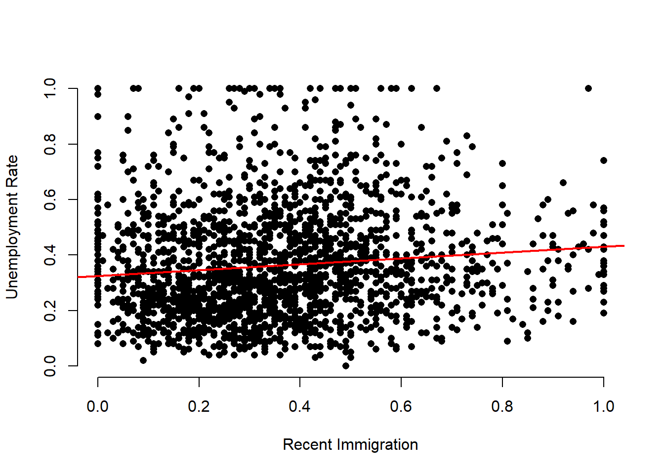
- How does this model compare to the models we estimated in the seminar with NoHighSchool and Minority as independent variables? Present your findings by comparing the output of all three models in side-by-side tables using the texreg package.
m_edu <- lm(unemploymentrate ~ nohighschool, data = com)

# minority percentage
com$minority <- 1 - com$white
m_minority <- lm(unemploymentrate ~ minority, data = com)

texreg::screenreg(list(m_edu, m_minority, m_immi))
##
## =========================================================
## Model 1 Model 2 Model 3
## ---------------------------------------------------------
## (Intercept) 0.08 *** 0.26 *** 0.33 ***
## (0.01) (0.01) (0.01)
## nohighschool 0.74 ***
## (0.01)
## minority 0.43 ***
## (0.02)
## recentimmigration5 0.11 ***
## (0.02)
## ---------------------------------------------------------
## R^2 0.55 0.27 0.01
## Adj. R^2 0.55 0.27 0.01
## Num. obs. 1994 1994 1994
## RMSE 0.14 0.17 0.20
## =========================================================
## *** p < 0.001, ** p < 0.01, * p < 0.05- Save your model comparison table to a Microsoft Word document (or another format if you don’t use Word).
texreg::htmlreg(list(m_edu, m_minority, m_immi), file = "Lab2_model_comparison.doc")## The table was written to the file 'Lab2_model_comparison.doc'.- Generate predicted values from the fitted model with RecentImmigration5 and plot the confidence interval using
Zelig.
library(Zelig)## Warning: package 'Zelig' was built under R version 3.4.1z.out <- zelig(unemploymentrate ~ recentimmigration5, data = com, model = "ls")## How to cite this model in Zelig:
## R Core Team. 2007.
## ls: Least Squares Regression for Continuous Dependent Variables
## in Christine Choirat, Christopher Gandrud, James Honaker, Kosuke Imai, Gary King, and Olivia Lau,
## "Zelig: Everyone's Statistical Software," http://zeligproject.org/x.out <- setx(z.out, recentimmigration5 = seq(0, 1, 0.1))
s.out <- sim(z.out, x = x.out, n=1000)- Save all the plots as graphics files.
png("task8_plot.png")
ci.plot(s.out, xlab = "Recent Immigration (last 5 years)", ci = 95)
dev.off()
## png
## 2