Lab 5 – Subset Selection
Philipp Broniecki and Lucas Leemann – Machine Learning 1K
(based on James et al. 2013, chapter 6)
We start by clearing our workspace.
# clear workspace
rm( list = ls() )
Subset Selection Methods
We use a modified data set on non-western immigrants (we inserted some missings). Download the data here.
The codebook is:
| Variable Name | Description |
|---|---|
| IMMBRIT | Out of every 100 people in Britain, how many do you think are immigrants from Non-western countries? |
| over.estimate | 1 if estimate is higher than 10.7%. |
| RSex | 1 = male, 2 = female |
| RAge | Age of respondent |
| Househld | Number of people living in respondent’s household |
| Cons, Lab, SNP, Ukip, BNP, GP, party.other | Party self-identification |
| paper | Do you normally read any daily morning newspaper 3+ times/week? |
| WWWhourspW | How many hours WWW per week? |
| religious | Do you regard yourself as belonging to any particular religion? |
| employMonths | How many mnths w. present employer? |
| urban | Population density, 4 categories (highest density is 4, lowest is 1) |
| health.good | How is your health in general for someone of your age? (0: bad, 1: fair, 2: fairly good, 3: good) |
| HHInc | Income bands for household, high number = high HH income |
# load foreigners data
load("your directory/BSAS_manip_missings.RData")
We check our data set for missing values variable by variable using apply(), is.na(), and table().
# check for missing values
apply(df, 2, function(x) table(is.na(x))["TRUE"] )
## IMMBRIT over.estimate RSex RAge Househld
## 8 NA NA NA NA
## Cons Lab SNP Ukip BNP
## NA NA NA NA NA
## GP party.other paper WWWhourspW religious
## NA NA NA NA NA
## employMonths urban health.good HHInc
## NA NA NA NA# we drop missings in IMMBRIT
df <- df[ !is.na(df$IMMBRIT), ]
# to drop variables on the entire dataset (uncomment next line)
#df <- na.omit(df)We now declare the categorical variables to be factors and create a copy of the main data set that excludes over.estimate.
# declare factor variables
df$urban <- factor(df$urban, labels = c("rural", "more rural", "more urban", "urban"))
df$RSex <- factor(df$RSex, labels = c("Male", "Female"))
df$health.good <- factor(df$health.good, labels = c("bad", "fair", "fairly good", "good") )

# drop the binary response coded 1 if IMMBRIT > 10.7
df$over.estimate <- NULL
df$Cons <- NULL
Best Subset Selection
We use the regsubsets() function to identify the best model based on subset selection quantified by the residual sum of squares (RSS) for each model.
library(leaps)

# run best subset selection
regfit.full <- regsubsets(IMMBRIT ~ ., data = df)
summary(regfit.full)
## Subset selection object
## Call: regsubsets.formula(IMMBRIT ~ ., data = df)
## 20 Variables (and intercept)
## Forced in Forced out
## RSexFemale FALSE FALSE
## RAge FALSE FALSE
## Househld FALSE FALSE
## Lab FALSE FALSE
## SNP FALSE FALSE
## Ukip FALSE FALSE
## BNP FALSE FALSE
## GP FALSE FALSE
## party.other FALSE FALSE
## paper FALSE FALSE
## WWWhourspW FALSE FALSE
## religious FALSE FALSE
## employMonths FALSE FALSE
## urbanmore rural FALSE FALSE
## urbanmore urban FALSE FALSE
## urbanurban FALSE FALSE
## health.goodfair FALSE FALSE
## health.goodfairly good FALSE FALSE
## health.goodgood FALSE FALSE
## HHInc FALSE FALSE
## 1 subsets of each size up to 8
## Selection Algorithm: exhaustive
## RSexFemale RAge Househld Lab SNP Ukip BNP GP party.other paper
## 1 ( 1 ) " " " " " " " " " " " " " " " " " " " "
## 2 ( 1 ) "*" " " " " " " " " " " " " " " " " " "
## 3 ( 1 ) "*" " " "*" " " " " " " " " " " " " " "
## 4 ( 1 ) "*" " " "*" " " " " " " "*" " " " " " "
## 5 ( 1 ) "*" " " "*" "*" " " " " "*" " " " " " "
## 6 ( 1 ) "*" "*" "*" "*" " " " " "*" " " " " " "
## 7 ( 1 ) "*" "*" "*" "*" " " " " "*" " " " " "*"
## 8 ( 1 ) "*" "*" "*" "*" " " "*" "*" " " " " "*"
## WWWhourspW religious employMonths urbanmore rural urbanmore urban
## 1 ( 1 ) " " " " " " " " " "
## 2 ( 1 ) " " " " " " " " " "
## 3 ( 1 ) " " " " " " " " " "
## 4 ( 1 ) " " " " " " " " " "
## 5 ( 1 ) " " " " " " " " " "
## 6 ( 1 ) " " " " " " " " " "
## 7 ( 1 ) " " " " " " " " " "
## 8 ( 1 ) " " " " " " " " " "
## urbanurban health.goodfair health.goodfairly good health.goodgood
## 1 ( 1 ) " " " " " " " "
## 2 ( 1 ) " " " " " " " "
## 3 ( 1 ) " " " " " " " "
## 4 ( 1 ) " " " " " " " "
## 5 ( 1 ) " " " " " " " "
## 6 ( 1 ) " " " " " " " "
## 7 ( 1 ) " " " " " " " "
## 8 ( 1 ) " " " " " " " "
## HHInc
## 1 ( 1 ) "*"
## 2 ( 1 ) "*"
## 3 ( 1 ) "*"
## 4 ( 1 ) "*"
## 5 ( 1 ) "*"
## 6 ( 1 ) "*"
## 7 ( 1 ) "*"
## 8 ( 1 ) "*"With the nvmax parameter we control the number of variables in the model. The default used by regsubsets() is 8.
# increase the max number of variables
regfit.full <- regsubsets(IMMBRIT ~ ., data = df, nvmax = 16)
reg.summary <- summary(regfit.full)
We can look at the components of the reg.summary object using the names() function and examine the \(R^2\) statistic stored in rsq.
names(reg.summary)## [1] "which" "rsq" "rss" "adjr2" "cp" "bic" "outmat" "obj"reg.summary$rsq## [1] 0.1040145 0.1316228 0.1469748 0.1546376 0.1595363 0.1621379 0.1650727
## [8] 0.1672137 0.1689371 0.1699393 0.1708328 0.1717100 0.1721041 0.1723151
## [15] 0.1725153 0.1726176Next, we plot the \(RSS\) and adjusted \(R^2\) and add a point where \(R^2\) is at its maximum using the which.max() function.
par( mfrow =  c(2,2) ) # 2 row, 2 columns in plot window
plot(reg.summary$rss, xlab = "Number of Variables", ylab = "Residual Sum of Squares", type = "l")
plot(reg.summary$adjr2, xlab = "Number of Variables", ylab = "Adjusted R^2", type = "l")

# find the peak of adj. R^2
adjr2.max <- which.max( reg.summary$adjr2 )
points(adjr2.max, reg.summary$adjr2[adjr2.max], col = "red", pch = 20, cex = 2)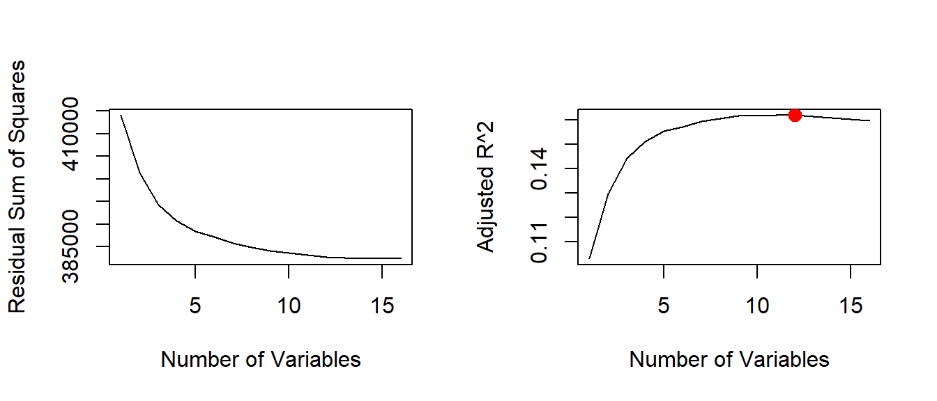
We can also plot the \(C_{p}\) statistic and \(BIC\) and identify the minimum points for each statistic using the \(which.min()\) function.
# cp
plot(reg.summary$cp, xlab = "Number of Variables", ylab = "Cp", type = "l")
cp.min <- which.min(reg.summary$cp)
points(cp.min, reg.summary$cp[cp.min], col = "red", cex = 2, pch = 20)

# bic
bic.min <- which.min(reg.summary$bic)
plot(reg.summary$bic, xlab = "Number of Variables", ylab = "BIC", type = "l")
points(bic.min, reg.summary$bic[bic.min], col = "red", cex = 2, pch = 20)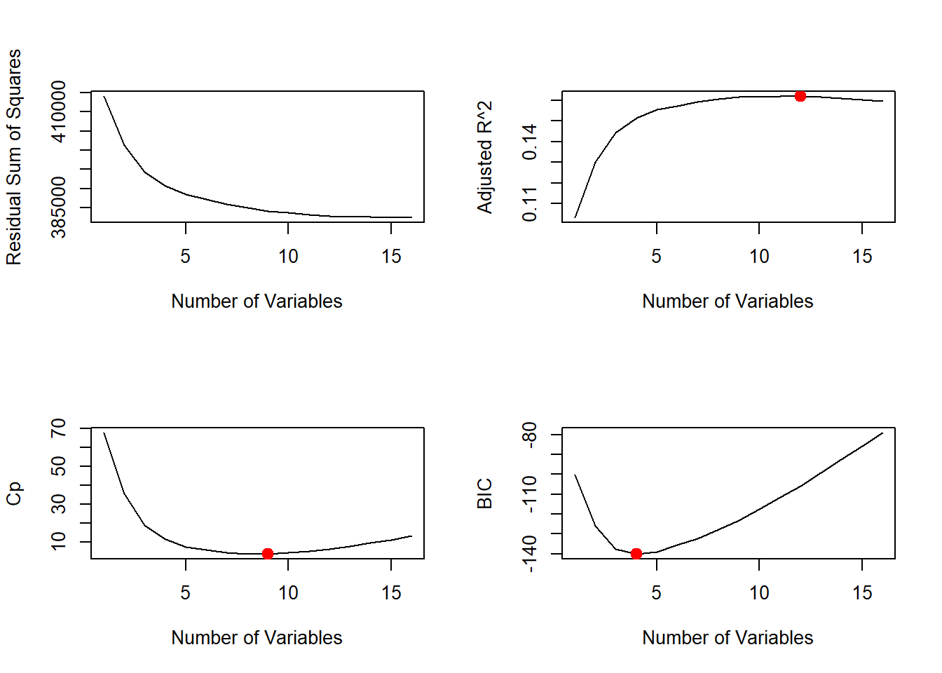
The estimated models from regsubsets() can be directly plotted to compare the differences based on the values of \(R^2\), adjusted \(R^2\), \(C_{p}\) and \(BIC\) statistics.
par( mfrow = c(1,1), oma = c(3,0,0,0))

# plot model comparison based on R^2
plot(regfit.full, scale = "r2")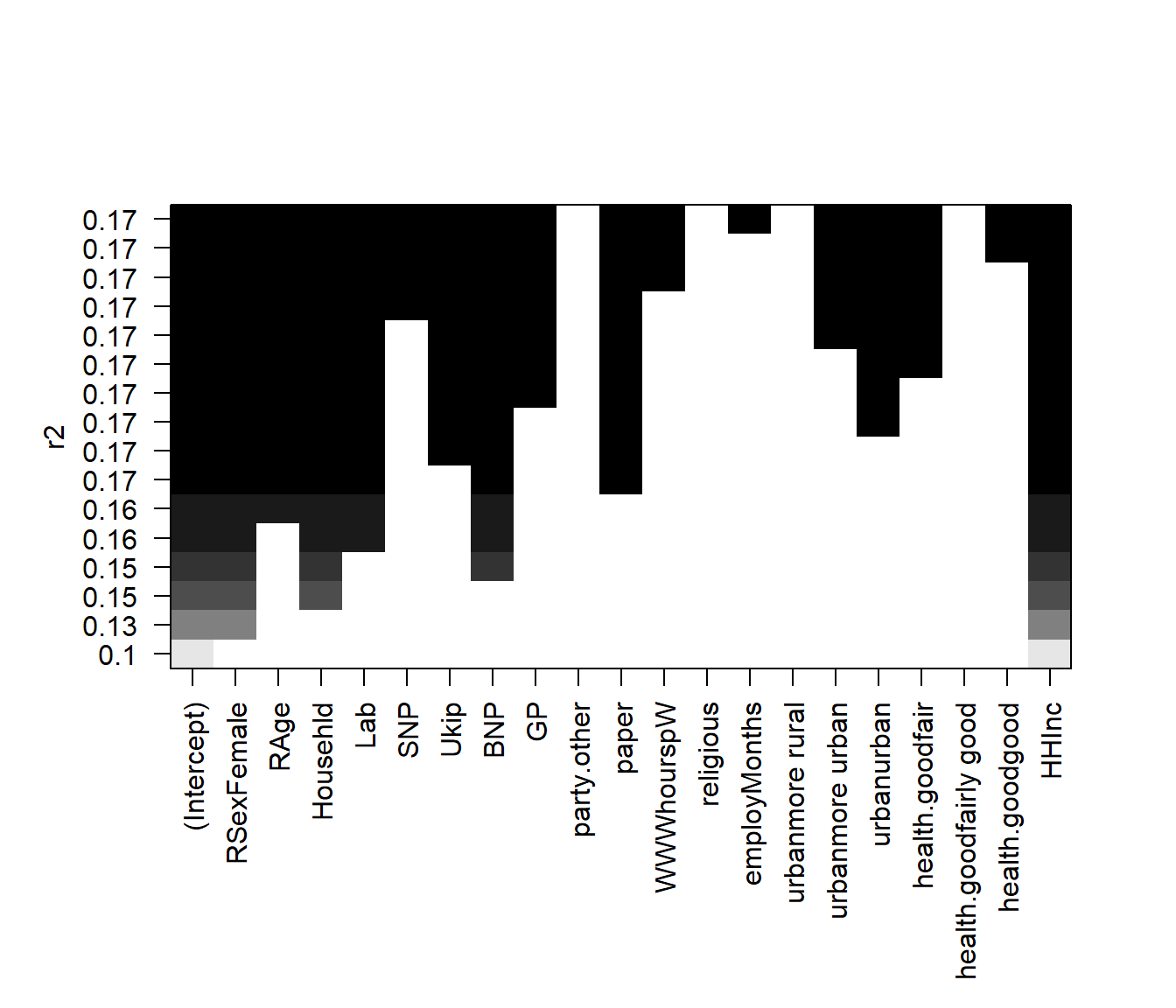
# plot model comparison based on adjusted R^2
plot(regfit.full, scale = "adjr2")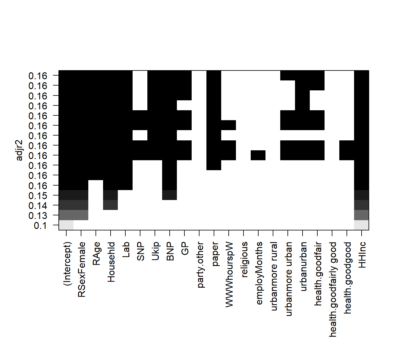
# plot model comparison based on adjusted CP
plot(regfit.full, scale = "Cp")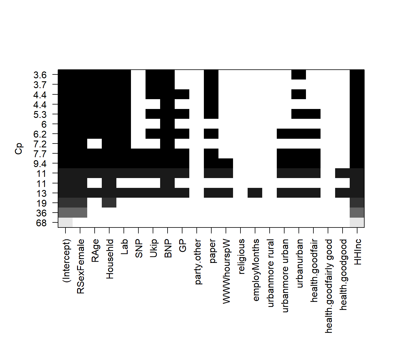
# plot model comparison based on adjusted BIC
plot(regfit.full, scale = "bic")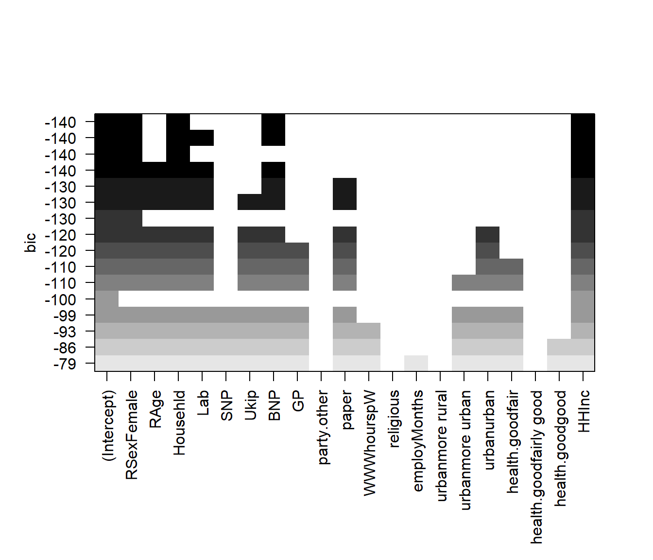
To show the coefficients associated with the model with the lowest \(BIC\), we use the coef() function.
coef(regfit.full, bic.min)## (Intercept) RSexFemale Househld BNP HHInc
## 34.576036 6.970692 2.000771 10.830195 -1.511176Forward and Backward Stepwise Selection
The default method used by regsubsets() is exhaustive but we can change it to forward or backward and compare the results.
# run forward selection
regfit.fwd <- regsubsets(IMMBRIT ~ ., data = df, nvmax = 16, method = "forward")
summary(regfit.fwd)
## Subset selection object
## Call: regsubsets.formula(IMMBRIT ~ ., data = df, nvmax = 16, method = "forward")
## 20 Variables (and intercept)
## Forced in Forced out
## RSexFemale FALSE FALSE
## RAge FALSE FALSE
## Househld FALSE FALSE
## Lab FALSE FALSE
## SNP FALSE FALSE
## Ukip FALSE FALSE
## BNP FALSE FALSE
## GP FALSE FALSE
## party.other FALSE FALSE
## paper FALSE FALSE
## WWWhourspW FALSE FALSE
## religious FALSE FALSE
## employMonths FALSE FALSE
## urbanmore rural FALSE FALSE
## urbanmore urban FALSE FALSE
## urbanurban FALSE FALSE
## health.goodfair FALSE FALSE
## health.goodfairly good FALSE FALSE
## health.goodgood FALSE FALSE
## HHInc FALSE FALSE
## 1 subsets of each size up to 16
## Selection Algorithm: forward
## RSexFemale RAge Househld Lab SNP Ukip BNP GP party.other paper
## 1 ( 1 ) " " " " " " " " " " " " " " " " " " " "
## 2 ( 1 ) "*" " " " " " " " " " " " " " " " " " "
## 3 ( 1 ) "*" " " "*" " " " " " " " " " " " " " "
## 4 ( 1 ) "*" " " "*" " " " " " " "*" " " " " " "
## 5 ( 1 ) "*" " " "*" "*" " " " " "*" " " " " " "
## 6 ( 1 ) "*" "*" "*" "*" " " " " "*" " " " " " "
## 7 ( 1 ) "*" "*" "*" "*" " " " " "*" " " " " "*"
## 8 ( 1 ) "*" "*" "*" "*" " " "*" "*" " " " " "*"
## 9 ( 1 ) "*" "*" "*" "*" " " "*" "*" " " " " "*"
## 10 ( 1 ) "*" "*" "*" "*" " " "*" "*" "*" " " "*"
## 11 ( 1 ) "*" "*" "*" "*" " " "*" "*" "*" " " "*"
## 12 ( 1 ) "*" "*" "*" "*" " " "*" "*" "*" " " "*"
## 13 ( 1 ) "*" "*" "*" "*" "*" "*" "*" "*" " " "*"
## 14 ( 1 ) "*" "*" "*" "*" "*" "*" "*" "*" " " "*"
## 15 ( 1 ) "*" "*" "*" "*" "*" "*" "*" "*" " " "*"
## 16 ( 1 ) "*" "*" "*" "*" "*" "*" "*" "*" " " "*"
## WWWhourspW religious employMonths urbanmore rural
## 1 ( 1 ) " " " " " " " "
## 2 ( 1 ) " " " " " " " "
## 3 ( 1 ) " " " " " " " "
## 4 ( 1 ) " " " " " " " "
## 5 ( 1 ) " " " " " " " "
## 6 ( 1 ) " " " " " " " "
## 7 ( 1 ) " " " " " " " "
## 8 ( 1 ) " " " " " " " "
## 9 ( 1 ) " " " " " " " "
## 10 ( 1 ) " " " " " " " "
## 11 ( 1 ) " " " " " " " "
## 12 ( 1 ) " " " " " " " "
## 13 ( 1 ) " " " " " " " "
## 14 ( 1 ) "*" " " " " " "
## 15 ( 1 ) "*" " " " " " "
## 16 ( 1 ) "*" " " "*" " "
## urbanmore urban urbanurban health.goodfair
## 1 ( 1 ) " " " " " "
## 2 ( 1 ) " " " " " "
## 3 ( 1 ) " " " " " "
## 4 ( 1 ) " " " " " "
## 5 ( 1 ) " " " " " "
## 6 ( 1 ) " " " " " "
## 7 ( 1 ) " " " " " "
## 8 ( 1 ) " " " " " "
## 9 ( 1 ) " " "*" " "
## 10 ( 1 ) " " "*" " "
## 11 ( 1 ) " " "*" "*"
## 12 ( 1 ) "*" "*" "*"
## 13 ( 1 ) "*" "*" "*"
## 14 ( 1 ) "*" "*" "*"
## 15 ( 1 ) "*" "*" "*"
## 16 ( 1 ) "*" "*" "*"
## health.goodfairly good health.goodgood HHInc
## 1 ( 1 ) " " " " "*"
## 2 ( 1 ) " " " " "*"
## 3 ( 1 ) " " " " "*"
## 4 ( 1 ) " " " " "*"
## 5 ( 1 ) " " " " "*"
## 6 ( 1 ) " " " " "*"
## 7 ( 1 ) " " " " "*"
## 8 ( 1 ) " " " " "*"
## 9 ( 1 ) " " " " "*"
## 10 ( 1 ) " " " " "*"
## 11 ( 1 ) " " " " "*"
## 12 ( 1 ) " " " " "*"
## 13 ( 1 ) " " " " "*"
## 14 ( 1 ) " " " " "*"
## 15 ( 1 ) " " "*" "*"
## 16 ( 1 ) " " "*" "*"# run backward selection
regfit.bwd <- regsubsets(IMMBRIT ~ ., data = df, nvmax = 16, method = "backward")
summary(regfit.bwd)## Subset selection object
## Call: regsubsets.formula(IMMBRIT ~ ., data = df, nvmax = 16, method = "backward")
## 20 Variables (and intercept)
## Forced in Forced out
## RSexFemale FALSE FALSE
## RAge FALSE FALSE
## Househld FALSE FALSE
## Lab FALSE FALSE
## SNP FALSE FALSE
## Ukip FALSE FALSE
## BNP FALSE FALSE
## GP FALSE FALSE
## party.other FALSE FALSE
## paper FALSE FALSE
## WWWhourspW FALSE FALSE
## religious FALSE FALSE
## employMonths FALSE FALSE
## urbanmore rural FALSE FALSE
## urbanmore urban FALSE FALSE
## urbanurban FALSE FALSE
## health.goodfair FALSE FALSE
## health.goodfairly good FALSE FALSE
## health.goodgood FALSE FALSE
## HHInc FALSE FALSE
## 1 subsets of each size up to 16
## Selection Algorithm: backward
## RSexFemale RAge Househld Lab SNP Ukip BNP GP party.other paper
## 1 ( 1 ) " " " " " " " " " " " " " " " " " " " "
## 2 ( 1 ) "*" " " " " " " " " " " " " " " " " " "
## 3 ( 1 ) "*" " " "*" " " " " " " " " " " " " " "
## 4 ( 1 ) "*" " " "*" " " " " " " "*" " " " " " "
## 5 ( 1 ) "*" " " "*" "*" " " " " "*" " " " " " "
## 6 ( 1 ) "*" "*" "*" "*" " " " " "*" " " " " " "
## 7 ( 1 ) "*" "*" "*" "*" " " " " "*" " " " " "*"
## 8 ( 1 ) "*" "*" "*" "*" " " "*" "*" " " " " "*"
## 9 ( 1 ) "*" "*" "*" "*" " " "*" "*" " " " " "*"
## 10 ( 1 ) "*" "*" "*" "*" " " "*" "*" "*" " " "*"
## 11 ( 1 ) "*" "*" "*" "*" " " "*" "*" "*" " " "*"
## 12 ( 1 ) "*" "*" "*" "*" " " "*" "*" "*" " " "*"
## 13 ( 1 ) "*" "*" "*" "*" "*" "*" "*" "*" " " "*"
## 14 ( 1 ) "*" "*" "*" "*" "*" "*" "*" "*" " " "*"
## 15 ( 1 ) "*" "*" "*" "*" "*" "*" "*" "*" " " "*"
## 16 ( 1 ) "*" "*" "*" "*" "*" "*" "*" "*" " " "*"
## WWWhourspW religious employMonths urbanmore rural
## 1 ( 1 ) " " " " " " " "
## 2 ( 1 ) " " " " " " " "
## 3 ( 1 ) " " " " " " " "
## 4 ( 1 ) " " " " " " " "
## 5 ( 1 ) " " " " " " " "
## 6 ( 1 ) " " " " " " " "
## 7 ( 1 ) " " " " " " " "
## 8 ( 1 ) " " " " " " " "
## 9 ( 1 ) " " " " " " " "
## 10 ( 1 ) " " " " " " " "
## 11 ( 1 ) " " " " " " " "
## 12 ( 1 ) " " " " " " " "
## 13 ( 1 ) " " " " " " " "
## 14 ( 1 ) "*" " " " " " "
## 15 ( 1 ) "*" " " " " " "
## 16 ( 1 ) "*" " " "*" " "
## urbanmore urban urbanurban health.goodfair
## 1 ( 1 ) " " " " " "
## 2 ( 1 ) " " " " " "
## 3 ( 1 ) " " " " " "
## 4 ( 1 ) " " " " " "
## 5 ( 1 ) " " " " " "
## 6 ( 1 ) " " " " " "
## 7 ( 1 ) " " " " " "
## 8 ( 1 ) " " " " " "
## 9 ( 1 ) " " "*" " "
## 10 ( 1 ) " " "*" " "
## 11 ( 1 ) " " "*" "*"
## 12 ( 1 ) "*" "*" "*"
## 13 ( 1 ) "*" "*" "*"
## 14 ( 1 ) "*" "*" "*"
## 15 ( 1 ) "*" "*" "*"
## 16 ( 1 ) "*" "*" "*"
## health.goodfairly good health.goodgood HHInc
## 1 ( 1 ) " " " " "*"
## 2 ( 1 ) " " " " "*"
## 3 ( 1 ) " " " " "*"
## 4 ( 1 ) " " " " "*"
## 5 ( 1 ) " " " " "*"
## 6 ( 1 ) " " " " "*"
## 7 ( 1 ) " " " " "*"
## 8 ( 1 ) " " " " "*"
## 9 ( 1 ) " " " " "*"
## 10 ( 1 ) " " " " "*"
## 11 ( 1 ) " " " " "*"
## 12 ( 1 ) " " " " "*"
## 13 ( 1 ) " " " " "*"
## 14 ( 1 ) " " " " "*"
## 15 ( 1 ) " " "*" "*"
## 16 ( 1 ) " " "*" "*"# mdoel coefficients of best 7-variable models
coef(regfit.full, 7)## (Intercept) RSexFemale RAge Househld Lab BNP
## 40.02553709 7.14423868 -0.08205116 1.70838328 -3.34664442 9.11326764
## paper HHInc
## 2.37633989 -1.60436490coef(regfit.fwd, 7)## (Intercept) RSexFemale RAge Househld Lab BNP
## 40.02553709 7.14423868 -0.08205116 1.70838328 -3.34664442 9.11326764
## paper HHInc
## 2.37633989 -1.60436490coef(regfit.bwd, 7)## (Intercept) RSexFemale RAge Househld Lab BNP
## 40.02553709 7.14423868 -0.08205116 1.70838328 -3.34664442 9.11326764
## paper HHInc
## 2.37633989 -1.60436490Choosing Among Models Using the Validation Set Approach and Cross-Validation
For validation set approach, we split the dataset into a training subset and a test subset. In order to ensure that the results are consistent over multiple iterations, we set the random seed with set.seed() before calling sample().
set.seed(1)

# sample true or false for each observation
train <- sample( c(TRUE, FALSE), size = nrow(df), replace = TRUE )
# the complement
test <- (!train)
We use regsubsets() as we did in the last section, but limit the estimation to the training subset.
regfit.best <- regsubsets(IMMBRIT ~ ., data = df[train, ], nvmax = 16)We create a matrix from the test subset using model.matrix(). Model matrix takes the dependent variable out of the data and adds an intercept to it.
# test data
test.mat <- model.matrix(IMMBRIT ~., data = df[test, ])
Next, we compute the validation error for each model.
# validation error for each model
val.errors <- NA
for (i in 1:16 ){
  coefi <- coef(regfit.best, id = i)
  y_hat <- test.mat[, names(coefi)] %*% coefi
  val.errors[i] <- mean(  (df$IMMBRIT[test] - y_hat)^2   )
}
We examine the validation error for each model and identify the best model with the lowest error.
val.errors## [1] 378.8917 383.0225 368.8723 372.9856 367.8958 371.1948 374.5266
## [8] 374.7800 374.4518 378.2256 376.5576 376.5623 375.7109 376.6845
## [15] 375.4616 375.3801# which model has smallest error
min.val.errors <- which.min(val.errors)
# coefficients of that model
coef( regfit.best, min.val.errors )## (Intercept) RSexFemale Househld BNP party.other HHInc
## 32.873751 5.199141 2.855654 8.450339 3.794634 -1.605292We can combine these steps into a function that can be called repeatedly when running k-fold cross-validation.
# precict function for repeatedly choosing model with lowest test error
predict.regsubsets <- function( object, newdata, id, ... ){
  # get the formula from the model
  m.formula <- as.formula( object$call[[2]] )
  # use that formula to create the model matrix for some new data
  mat <- model.matrix( m.formula, newdata )
  # get coeffiecients where id is the number of variables
  coefi <- coef( object, id = id )
  # get the variable names of current model
  xvars <- names( coefi )
  # multiply data with coefficients
  mat[ , xvars ] %*% coefi
}
We run regsubsets() on the full dataset and examine the coefficients associated with the model that has the lower validation error.
# best subset on full data set
regfit.best <- regsubsets( IMMBRIT ~ ., data = df, nvmax = 16 )

# examine coefficients of the model that had the lowest validation error
coef( regfit.best, min.val.errors )
## (Intercept) RSexFemale Househld Lab BNP HHInc
## 35.920518 6.886259 2.062351 -3.394188 9.708402 -1.563859k-fold cross-validation
For cross-validation, we create the number of folds needed (10, in this case) and allocate a matrix for storing the results.
# number of folds
k <- 10
set.seed(1)
# fold assignment for each observation
folds <- sample(1:k, nrow(df), replace = TRUE)
# frequency table of fold assignment (should be relatively balanced)
table(folds)
## folds
## 1 2 3 4 5 6 7 8 9 10
## 99 110 97 116 117 93 93 108 94 114# container for cross-validation errors
cv.errors <- matrix(NA, nrow = k, ncol = 16, dimnames = list(NULL, paste(1:16)))
# have a look at the matrix
cv.errors## 1 2 3 4 5 6 7 8 9 10 11 12 13 14 15 16
## [1,] NA NA NA NA NA NA NA NA NA NA NA NA NA NA NA NA
## [2,] NA NA NA NA NA NA NA NA NA NA NA NA NA NA NA NA
## [3,] NA NA NA NA NA NA NA NA NA NA NA NA NA NA NA NA
## [4,] NA NA NA NA NA NA NA NA NA NA NA NA NA NA NA NA
## [5,] NA NA NA NA NA NA NA NA NA NA NA NA NA NA NA NA
## [6,] NA NA NA NA NA NA NA NA NA NA NA NA NA NA NA NA
## [7,] NA NA NA NA NA NA NA NA NA NA NA NA NA NA NA NA
## [8,] NA NA NA NA NA NA NA NA NA NA NA NA NA NA NA NA
## [9,] NA NA NA NA NA NA NA NA NA NA NA NA NA NA NA NA
## [10,] NA NA NA NA NA NA NA NA NA NA NA NA NA NA NA NAWe then run through each fold in a for() loop and predict the salary using our predict function. We then calculate the validation error for each fold and save them in the matrix created above.
# loop over folds
for (a in 1:k){

  # best subset selection on training data
  best.fit <- regsubsets(IMMBRIT ~ ., data = df[ folds != a, ], nvmax = 16)

  # loop over the 16 subsets
  for (b in 1:16){

    # predict response for test set for current subset
    pred <- predict(best.fit, df[ folds == a ,], id = b )

    # MSE into container; rows are folds; columns are subsets
    cv.errors[a, b] <- mean( (df$IMMBRIT[folds==a] - pred)^2 )

  } # end of loop over the 16 subsets
} # end of loop over folds
# the cross-validation error matrix
cv.errors
## 1 2 3 4 5 6 7
## [1,] 358.7386 334.5939 323.8124 317.4231 311.8484 316.8302 315.0793
## [2,] 379.2802 376.4512 389.1254 374.1665 383.3341 380.6665 380.3079
## [3,] 442.9207 426.1023 412.6952 421.7677 418.0278 423.1556 425.7611
## [4,] 439.7298 437.2049 416.2253 423.5752 421.0708 424.7605 428.6010
## [5,] 459.3967 456.7258 446.3888 447.3912 443.2314 453.3881 459.1921
## [6,] 383.8459 366.5701 365.7940 377.7461 372.7480 372.1247 366.5200
## [7,] 361.8168 345.1388 352.6694 351.2537 339.6718 337.8319 335.8549
## [8,] 411.4885 400.3470 395.9349 383.9394 395.3248 386.5663 386.2542
## [9,] 424.7996 398.0276 380.7486 379.0400 377.4007 366.7923 362.5681
## [10,] 321.5108 317.1196 337.1115 347.0513 341.4610 341.8680 344.7225
## 8 9 10 11 12 13 14
## [1,] 315.1698 315.7354 316.5184 316.1405 318.2277 317.6919 317.6408
## [2,] 385.5818 386.1221 387.0886 387.2579 390.6045 391.3079 391.6435
## [3,] 429.8113 429.5870 427.2789 427.0476 421.5395 420.3084 421.8910
## [4,] 429.9591 436.7310 438.4459 432.5970 436.2287 434.4739 434.3651
## [5,] 458.8809 461.2268 451.4365 453.6881 458.8213 457.3609 459.5737
## [6,] 365.4540 367.0784 363.6070 362.8737 363.1972 361.1425 364.8936
## [7,] 333.5200 333.5632 334.1020 330.4406 329.3324 329.9864 331.1112
## [8,] 379.9411 379.1488 379.5117 379.5639 376.7432 376.7048 374.5593
## [9,] 363.4348 369.9028 366.8833 367.5859 375.8546 380.4760 380.8302
## [10,] 342.6951 341.4322 338.6518 337.1286 335.1587 335.8101 336.3503
## 15 16
## [1,] 317.6161 317.8835
## [2,] 390.7027 391.5483
## [3,] 420.6856 421.4002
## [4,] 436.6631 436.7150
## [5,] 458.9685 460.2302
## [6,] 367.5902 367.0877
## [7,] 331.0008 330.4741
## [8,] 374.7864 376.7694
## [9,] 382.5580 385.0165
## [10,] 337.3890 336.5040We calculate the mean error for all subsets by applying mean to each column using the apply() function.
# average cross-validation errors over the folds
mean.cv.errors <- apply(cv.errors, 2, mean)
mean.cv.errors
## 1 2 3 4 5 6 7 8
## 398.3527 385.8281 382.0506 382.3354 380.4119 380.3984 380.4861 380.4448
## 9 10 11 12 13 14 15 16
## 382.0528 380.3524 379.4324 380.5708 380.5263 381.2859 381.7960 382.3629# visualize
par( mfrow = c(1,1) , oma = c(0,0,0,0))
plot( mean.cv.errors, type = "b" )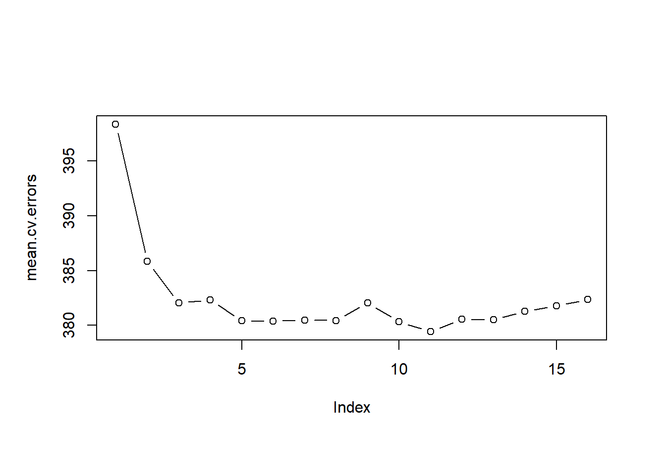
Finally, we run regsubsets() on the full dataset and show the coefficients for the best performing model which we picked using 10-fold cross-validation.
# run regsubsets on full data set
reg.best <- regsubsets(IMMBRIT ~ ., data = df, nvmax = 16)
# coefficients of subset which minimized test error
coef(reg.best, which.min(mean.cv.errors))
## (Intercept) RSexFemale RAge Househld
## 39.77322361 7.01819910 -0.07375744 1.73379158
## Lab Ukip BNP GP
## -3.93833149 -6.00319269 9.20444619 -4.52952484
## paper urbanurban health.goodfair HHInc
## 2.43834361 2.17126407 -1.72574453 -1.60450935Exercises
Q1
In this exercise, we will generate simulated data, and will then use this data to perform best subset selection.
- Use the
rnorm()function to generate a predictor \(X\) of length \(n=100\), as well as a noise vector \(\epsilon\) of length \(n=100\). - Generate a response vector \(Y\) of length \(n=100\) according to the model \[ Y = \beta_{0} + \beta_{1} X + \beta_{2} X^{2} + \beta_{3} X^{3} + \epsilon,\] where \(\beta_{0},\: \beta_{1}, \: \beta_{2}, \: \beta_{3}\) are constants of your choice.
- Use the
regsubsets()function to perform best subset selection in order to choose the best model containing the predictors \(X, X^2,\ldots,X^{10}\). What is the best model obtained according to \(C_{p}\), \(BIC\), and adjusted \(R^2\) Show some plots to provide evidence for your answer, and report the coefficients of the best model obtained. Note you will need to use thedata.frame()function to create a single data set containing both \(X\) and \(Y\). - Repeat (3), using forward stepwise selection and also using backwards stepwise selection. How does your answer compare to the results in (3)?
Q2
We have seen that as the number of features used in a model increases, the training error will necessarily decrease, but the test error may not. We will now explore this in a simulated data set.
- Generate a data set with \(p=20\) features, \(n=1,000\) observations, and an associated quantitative response vector generated according to the model \[Y = X\beta+\epsilon,\] where \(\beta\) has some elements that are exactly equal to \(0\).
- Split your dataset into a training set containing \(100\) observations and a test set containing \(900\) observations.
- Perform best subset selection on the training set, and plot the training set MSE associated with the best model of each size.
- Plot the test set MSE associated with the best model of each size.
- For which model size does the test set MSE take on its minimum value? Comment on your results. If it takes on its minimum value for a model containing only an intercept or a model containing all of the features, then play around with the way that you are generating the data in 1. until you come up with a scenario in which the test set MSE is minimized for an intermediate model size.