Solution Day 4 - Resampling Methods
Philipp Broniecki and Lucas Leemann – Machine Learning 1K
Q1
Load the full data set.
load("./data/BSAS_manip.RData")
df <- data2 # make copy with shorter name
rm(data2) # remove original- Fit a logistic regression model that uses
RSex,urban, andHHIncto predictover.estimate.
Note, RSex and urban are categorical variables. Categorical variables with more than 2 categories have to be declared factor variables or broken up into dummy variables manually. We show both below but breaking up RSex is not necessary because it has only 2 categories.
# declaring factor
df$urban <- factor(df$urban, labels = c("rural", "partly rural", "partly urban", "urban"))

# manual dummy coding
df$female <- ifelse(df$RSex == 2, yes = 1, no = 0)

set.seed(666)
glm.fit <- glm(over.estimate ~ female + urban + HHInc, data = df, family = binomial(link = "logit"))
summary(glm.fit)
##
## Call:
## glm(formula = over.estimate ~ female + urban + HHInc, family = binomial(link = "logit"),
## data = df)
##
## Deviance Residuals:
## Min 1Q Median 3Q Max
## -2.1204 -1.1808 0.6304 0.8285 1.2889
##
## Coefficients:
## Estimate Std. Error z value Pr(>|z|)
## (Intercept) 1.56226 0.24685 6.329 2.47e-10 ***
## female 0.58640 0.14355 4.085 4.41e-05 ***
## urbanpartly rural -0.05894 0.20121 -0.293 0.7696
## urbanpartly urban 0.29876 0.20443 1.461 0.1439
## urbanurban 0.36467 0.21759 1.676 0.0937 .
## HHInc -0.10362 0.01600 -6.477 9.34e-11 ***
## ---
## Signif. codes: 0 '***' 0.001 '**' 0.01 '*' 0.05 '.' 0.1 ' ' 1
##
## (Dispersion parameter for binomial family taken to be 1)
##
## Null deviance: 1236.9 on 1048 degrees of freedom
## Residual deviance: 1161.4 on 1043 degrees of freedom
## AIC: 1173.4
##
## Number of Fisher Scoring iterations: 4- Using the validation set approach, estimate the test error of this model. In order to do this, you must perform the following steps:
- Split the sample set into a training set and a validation set.
- Fit a multiple logistic regression model using only the training observations.
- Obtain a prediction for each individual in the validation set by computing the posterior probability of over estimating for that individual, and classifying the individual to the over estimating category if the posterior probability is greater than 0.5.
- Compute the validation set error, which is the fraction of the observations in the validation set that are misclassified.
val.err <- function(df){

  # a.
  train <- sample(nrow(df), size = nrow(df) *.5, replace = FALSE )

  # b.
  m <- glm(over.estimate ~ female + urban + HHInc, data = df,
           family = binomial(link = "logit"), subset = train)

  # c.
  p <- predict(m, newdata = df[-train,], type = "response")
  out <- ifelse( p > 0.5, yes = 1, no = 0)

  # d.
  return( mean( out != df$over.estimate[-train]) )
}

# call the function (the only argument it needs is the name of the data set)
val.err( df = df)
## [1] 0.2628571The error rate in the test set is \(25\%\).
- Repeat the process in (2) three times, using three different splits of the observations into a training set and a validation set. Comment on the results obtained.
for (a in 1:3) print(val.err( df = df))## [1] 0.28
## [1] 0.2457143
## [1] 0.2971429The error rate averages to roughly \(27\%\) in the three trials.
- Now consider a logistic regression model that predicts the probability of over estimating using additional dummy variables for people who self-identify with Ukip or the BNP. Estimate the test error for this model using the validation set approach. Comment on whether or not including dummy variables for Ukip and BNP leads to a reduction in the test error rate.
train <- sample(nrow(df), size = nrow(df) *.5, replace = FALSE)
m2 <- glm(over.estimate ~ female + urban + HHInc + Ukip + BNP,
          data = df, family = binomial, subset = train)
p <- predict( m2, newdata = df[-train, ], type = "response")
out <- ifelse( p > 0.5, yes = 1, no = 0)
mean( out != df$over.estimate[-train] )
## [1] 0.2914286The error rate remains at roughly \(27\%\). Adding the two dummies did not appear to improve prediction accuracy.
Q2
- Fit a logistic regression model on
over.estimateusingpaperandreligious.
m1 <- glm(over.estimate ~ paper + religious, data = df, family = binomial)
summary(m1)
##
## Call:
## glm(formula = over.estimate ~ paper + religious, family = binomial,
## data = df)
##
## Deviance Residuals:
## Min 1Q Median 3Q Max
## -1.6602 -1.5519 0.7734 0.8325 0.8445
##
## Coefficients:
## Estimate Std. Error z value Pr(>|z|)
## (Intercept) 0.84767 0.11092 7.642 2.13e-14 ***
## paper 0.03381 0.13939 0.243 0.808
## religious 0.20616 0.13890 1.484 0.138
## ---
## Signif. codes: 0 '***' 0.001 '**' 0.01 '*' 0.05 '.' 0.1 ' ' 1
##
## (Dispersion parameter for binomial family taken to be 1)
##
## Null deviance: 1236.9 on 1048 degrees of freedom
## Residual deviance: 1234.6 on 1046 degrees of freedom
## AIC: 1240.6
##
## Number of Fisher Scoring iterations: 4- Fit a logistic regression model that predicts
over.estimateusingpaperandreligioususing all but the first observation.
m2 <- glm(over.estimate ~ paper + religious, data = df[-1, ], family = binomial)
summary(m2)
##
## Call:
## glm(formula = over.estimate ~ paper + religious, family = binomial,
## data = df[-1, ])
##
## Deviance Residuals:
## Min 1Q Median 3Q Max
## -1.6589 -1.5558 0.7725 0.8315 0.8414
##
## Coefficients:
## Estimate Std. Error z value Pr(>|z|)
## (Intercept) 0.85632 0.11122 7.699 1.37e-14 ***
## paper 0.02819 0.13951 0.202 0.84
## religious 0.20027 0.13903 1.440 0.15
## ---
## Signif. codes: 0 '***' 0.001 '**' 0.01 '*' 0.05 '.' 0.1 ' ' 1
##
## (Dispersion parameter for binomial family taken to be 1)
##
## Null deviance: 1234.3 on 1047 degrees of freedom
## Residual deviance: 1232.2 on 1045 degrees of freedom
## AIC: 1238.2
##
## Number of Fisher Scoring iterations: 4- Use the model from (2) to predict the direction of the first observation. You can do this by predicting that the first observation will over estimate if \(P(over.estimate == 1 | paper, religious) > 0.5\). Was this observation correctly classified?
p <- predict(m2, newdata = df[1,], type = "response")
out <- ifelse( p > 0.5, yes = 1, no = 0)
out == df$over.estimate[1]
## 1
## FALSEThe first observation was classified incorrectly.
Write a for loop from \(i=1\) to \(i=n\), where \(n\) is the number of observations in the data set, that performs each of the following steps:
- Fit a logistic regression model using all but the \(i^{th}\) observation to predict
over.estimateusingpaperandreligious. - Compute the posterior probability that the person over-estimates the rate of immigrants for the \(i^{th}\) observation.
- Use the posterior probability for the \(i^{th}\) observation in order to predict whether or not the person over-estimates the rate of immigrants.
- Determine whether or not an error was made in predicting the direction for the \(i^{th}\) observation. If an error was made, then indicate this as a \(1\), and otherwise indicate it as a \(0\).
- Fit a logistic regression model using all but the \(i^{th}\) observation to predict
pred.all <- function(df, idx){

  # a.
  m <- glm(over.estimate ~ paper + religious, data = df[-idx,], family = binomial)

  # b.
  p <- predict(m, newdata = df[idx, ], type = "response")

  # c.
  exp.out <- ifelse( p > 0.5, yes = 1, no = 0)

  # d.
  return(ifelse( exp.out != df$over.estimate[idx], yes = 1, no = 0))
}

n.misclassifications <- 0
for (a in 1: nrow(df)) n.misclassifications <- n.misclassifications + pred.all(df, a)
n.misclassifications
## 1
## 290We make 290 errors.
- Take the average of the n numbers obtained in 4.d. in order to obtain the LOOCV estimate for the test error. Comment on the results.
n.misclassifications / nrow(df)## 1
## 0.2764538We misclassify \(28\%\) of the cases according to LOOCV.
Q3
- Generate a simulated data set as follows:
set.seed(1)
y <- rnorm(100)
x <- rnorm(100)
y <- x -2*x^2 + rnorm(100)
In this data set, what is \(n\) and what is \(p\)? Write out the model used to generate the data in equation form.
\(n = 100\), \(p = 2\); \(Y=X-2X^{2}+\epsilon\)
- Create a scatterplot of \(X\) against \(Y\). Comment on what you find.
plot( y ~ x, bty = "n", pch = 20)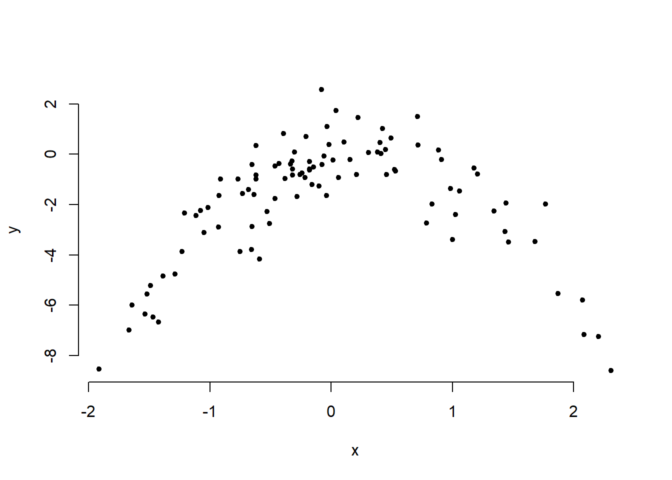
Quadratic plot. \(X\) from about \(-2\) to \(2\). \(Y\) from about \(-8\) to \(2\).
Set a random seed, and then compute the LOOCV errors that result from fitting the following four models using least squares:
- \(Y=\beta_{0}+\beta_{1}X+\epsilon\)
- \(Y=\beta_{0}+\beta_{1}X+\beta_{2}X_{2}+\epsilon\)
- \(Y=\beta_{0}+\beta_{1}X+\beta_{2}X_{2}+\beta_{3}X_{3}+\epsilon\)
- \(Y=\beta_{0}+\beta_{1}X+\beta_{2}X_{2}+\beta_{3}X_{3}+\beta_{4}X_{4}+\epsilon\)
Note, you may find it helpful to use the data.frame() function to create a single data set containing both \(X\) and \(Y\).
library(boot)
dat <- data.frame(x,y)
set.seed(1)

# a.
m <- glm(y ~ x)
cv.glm( dat, m)$delta
## [1] 5.890979 5.888812# b.
m <- glm( y ~ poly(x,2))
cv.glm(dat, m)$delta## [1] 1.086596 1.086326# c.
m <- glm( y ~ poly(x, 3) )
cv.glm(dat, m)$delta## [1] 1.102585 1.102227# d.
m <- glm( y ~ poly(x, 4) )
cv.glm( dat, m)$delta## [1] 1.114772 1.114334- Repeat the last task using another random seed, and report your results. Are your results the same as what you got 3.? Why?
set.seed(10)

# a.
m <- glm(y ~ x)
cv.glm( dat, m)$delta
## [1] 5.890979 5.888812# b.
m <- glm( y ~ poly(x,2))
cv.glm(dat, m)$delta## [1] 1.086596 1.086326# c.
m <- glm( y ~ poly(x, 3) )
cv.glm(dat, m)$delta## [1] 1.102585 1.102227# d.
m <- glm( y ~ poly(x, 4) )
cv.glm( dat, m)$delta## [1] 1.114772 1.114334Exact same, because LOOCV will be the same since it evaluates \(n\) folds of a single observation.
- Which of the models in 3. had the smallest LOOCV error? Is this what you expected? Explain your answer.
The quadratic polynomial had the lowest LOOCV test error rate. This was expected because it matches the true form of \(Y\).
- Comment on the statistical significance of the coefficient estimates that results from fitting each of the models in 3. using least squares. Do these results agree with the conclusions drawn based on the cross-validation results?
summary(m)##
## Call:
## glm(formula = y ~ poly(x, 4))
##
## Deviance Residuals:
## Min 1Q Median 3Q Max
## -2.8914 -0.5244 0.0749 0.5932 2.7796
##
## Coefficients:
## Estimate Std. Error t value Pr(>|t|)
## (Intercept) -1.8277 0.1041 -17.549 <2e-16 ***
## poly(x, 4)1 2.3164 1.0415 2.224 0.0285 *
## poly(x, 4)2 -21.0586 1.0415 -20.220 <2e-16 ***
## poly(x, 4)3 -0.3048 1.0415 -0.293 0.7704
## poly(x, 4)4 -0.4926 1.0415 -0.473 0.6373
## ---
## Signif. codes: 0 '***' 0.001 '**' 0.01 '*' 0.05 '.' 0.1 ' ' 1
##
## (Dispersion parameter for gaussian family taken to be 1.084654)
##
## Null deviance: 552.21 on 99 degrees of freedom
## Residual deviance: 103.04 on 95 degrees of freedom
## AIC: 298.78
##
## Number of Fisher Scoring iterations: 2p-values show statistical significance of linear and quadratic terms, which agrees with the CV results.