Lab 1 – Solutions

R Introduction (based on Leemann and Mykhaylov, PUBLG100)

2. Clear the workspace and set the working directory to your StatisticalLearning folder.

# clear workspace
rm( list = ls() )

We set the working directory with setwd(). You can find a detailed description here.

setwd("C:/some folder/some folder/StatisticalLearning")

3. Load the High School and Beyond dataset. Remember to load any necessary packages.

setwd("C:/Users/phili/Documents/ML2017.io")
library(readxl)

## Warning: package 'readxl' was built under R version 3.4.1

df <- read_excel("./data/hsb2.xlsx")

4. Calculate the final score for each student by averaging the read, write, math, science, and socst scores and save it in a column called final_score.

We use the apply() function. Check its helpfiles by typing ?apply. We pass a subset of our dataset only including the 5 variables to apply(). The second argument 1 tells apply() to work rowwise. The third argument tells it to take the mean.

df$final_score <- apply(df[, c("read", "write", "math", "science", "socst")], 1, mean)

5. Calculate the mean, median and mode for the final_score.

mean(df$final_score)

## [1] 52.384

median(df$final_score)

## [1] 53

There is no function for the mode. So we look at a frequency table of the final_score using the table() function. We put this inside the which.max() function which returns the index of the most frequent score. Finally, we index the frequency table with the id we obtained.

id.of.mode <- which.max(table(df$final_score))
table(df$final_score)[id.of.mode]

## 50.6 
##    5

6. Create a factor variable called school_type from schtyp using the following codes:
   • 1 = Public schools
   • 2 = Private schools

df$schtyp <- factor(df$schtyp, labels = c("Public schools", "Private schools"))

7. How many students are from private schools and how many are from public schools?

We again use the table() function to produce a frequency table.

table(df$schtyp)

## 
##  Public schools Private schools 
##             168              32

8. Calculate the variance and standard deviation for final_score from each school type.

Do do this we index the data with the square brackets. Inside we put a condition. Only the data where the condition is true will be evaluated. The double equal signs mean is the same

# variance
var(df$final_score[df$schtyp == "Private schools"])

## [1] 41.10645

var(df$final_score[df$schtyp == "Public schools"])

## [1] 70.97955

# standard deviation
sd(df$final_score[df$schtyp == "Private schools"])

## [1] 6.411431

sd(df$final_score[df$schtyp == "Public schools"])

## [1] 8.424936

9. Find out the ID of the students with the highest and lowest final_score from each school type.

We use the which.min() and which.max() functions again to get the index numbers of the correct students.

# best student's id from private school
df$id[ which.max(df$final_score[ df$schtyp == "Private schools" ]) ]

## [1] 76

# best student's id from public school
df$id[ which.max(df$final_score[ df$schtyp == "Private schools" ]) ]

## [1] 76

# worst student's id from private school
df$id[ which.min(df$final_score[df$schtyp == "Private schools"])]

## [1] 86

# worst student's id from private school
df$id[ which.min(df$final_score[df$schtyp == "Public schools"])]

## [1] 162

10. Find out the 20th, 40th, 60th and 80th percentiles of final_score.

The quantile() function allows us to do this easily.

quantile(df$final_score, c(.2, .4, .6, .8))

##   20%   40%   60%   80% 
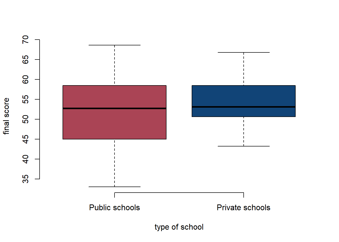
## 44.56 50.44 54.68 59.48

12. Create box plot for final_score grouped by the school_type factor variable to show the difference between final_score at public schools vs. private schools.

The plot() function knows that a boxplot is appropriate becuase schtyp is a factor variable.

plot(final_score ~ schtyp, data = df, bty = "l", col = c("#AA4455", "#114477"), 
     xlab = "type of school", ylab = "final score", frame.plot = FALSE)