Lab 6 – Regularization
Philipp Broniecki and Lucas Leemann – Machine Learning 1K
(based on James et al. 2013, chapter 6)
Ridge Regression and the Lasso
We start by clearing our workspace, loading the foreigners data, and doing the necessary variable manipulations. The data is available here.
# clear workspace
rm(list=ls())

# load foreigners data
load("your directory/BSAS_manip.RData")
head(data2)

# we declare the factor variables
data2$urban <- factor(data2$urban, labels = c("rural", "more rural", "more urban", "urban"))
data2$RSex <- factor(data2$RSex, labels = c("Male", "Female"))
data2$health.good <- factor(data2$health.good, labels = c("bad", "fair", "fairly good", "good") )

# categorical variables
cat.vars <- unlist(lapply(data2, function(x) is.factor(x) | all(x == 0 | x==1) | all( x==1 | x==2) ))
# normalize numeric variables
data2[, !cat.vars] <- apply(data2[, !cat.vars], 2, scale)
In order to run ridge regression, we create a matrix from our dataset using the model.matrix() function. We also need to remove the intercept from the resulting matrix because the function to run ridge regression automatically includes one. Furthermore, we will use the subjective rate of immigrants as response. Consequently, we have to remove over.estimate as it measures the same thing. Lastly, the party affiliation dummies are mutually exclusive, se we have to exclude the model category Cons.
# covariates in matrix form but remove the intercept, over.estimate, and Cons
x <- model.matrix(IMMBRIT ~ . -1 -over.estimate -Cons, data2)
# check if it looks fine
head(x)
## RSexMale RSexFemale RAge Househld Lab SNP Ukip BNP GP
## 1 1 0 0.0144845 -0.2925308 1 0 0 0 0
## 2 0 1 -1.8065476 0.4540989 0 0 0 0 0
## 3 0 1 0.5835570 -1.0391604 0 0 0 0 0
## 4 0 1 1.5509804 -0.2925308 0 0 0 0 0
## 5 0 1 0.9819078 -1.0391604 0 0 0 0 0
## 6 1 0 -1.1236606 1.2007285 0 0 0 0 0
## party.other paper WWWhourspW religious employMonths urbanmore rural
## 1 0 0 -0.5324636 0 -0.203378 0
## 2 1 0 -0.1566702 0 -0.203378 0
## 3 1 0 -0.5324636 0 5.158836 0
## 4 1 1 -0.4071991 1 -0.203378 0
## 5 1 0 -0.5324636 1 -0.203378 0
## 6 1 1 1.0959747 0 -0.203378 0
## urbanmore urban urbanurban health.goodfair health.goodfairly good
## 1 0 1 1 0
## 2 0 1 0 1
## 3 1 0 0 0
## 4 0 0 0 0
## 5 1 0 0 0
## 6 0 0 0 1
## health.goodgood HHInc
## 1 0 0.7357918
## 2 0 -1.4195993
## 3 1 -0.1263647
## 4 1 -0.3419038
## 5 1 -0.1263647
## 6 0 -0.1263647# response vector
y <- data2$IMMBRITRidge Regression
The glmnet package provides functionality to fit ridge regression and lasso models. We load the package and call glmnet() to perform ridge regression.
library(glmnet)

# tuning parameter
grid <- 10^seq(4, -2, length = 100)
plot(grid, bty = "n", pch = 19,
     main = expression(paste("Grid of Tuning Parameters ", lambda)))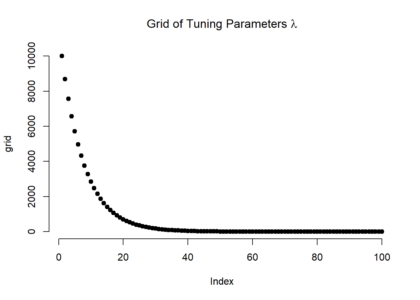
# run ridge; alpha = 0 means do ridge
ridge.mod <- glmnet(x, y, alpha = 0, lambda = grid)

# coefficient shrinkage visualized
plot(ridge.mod, xvar = "lambda", label = TRUE)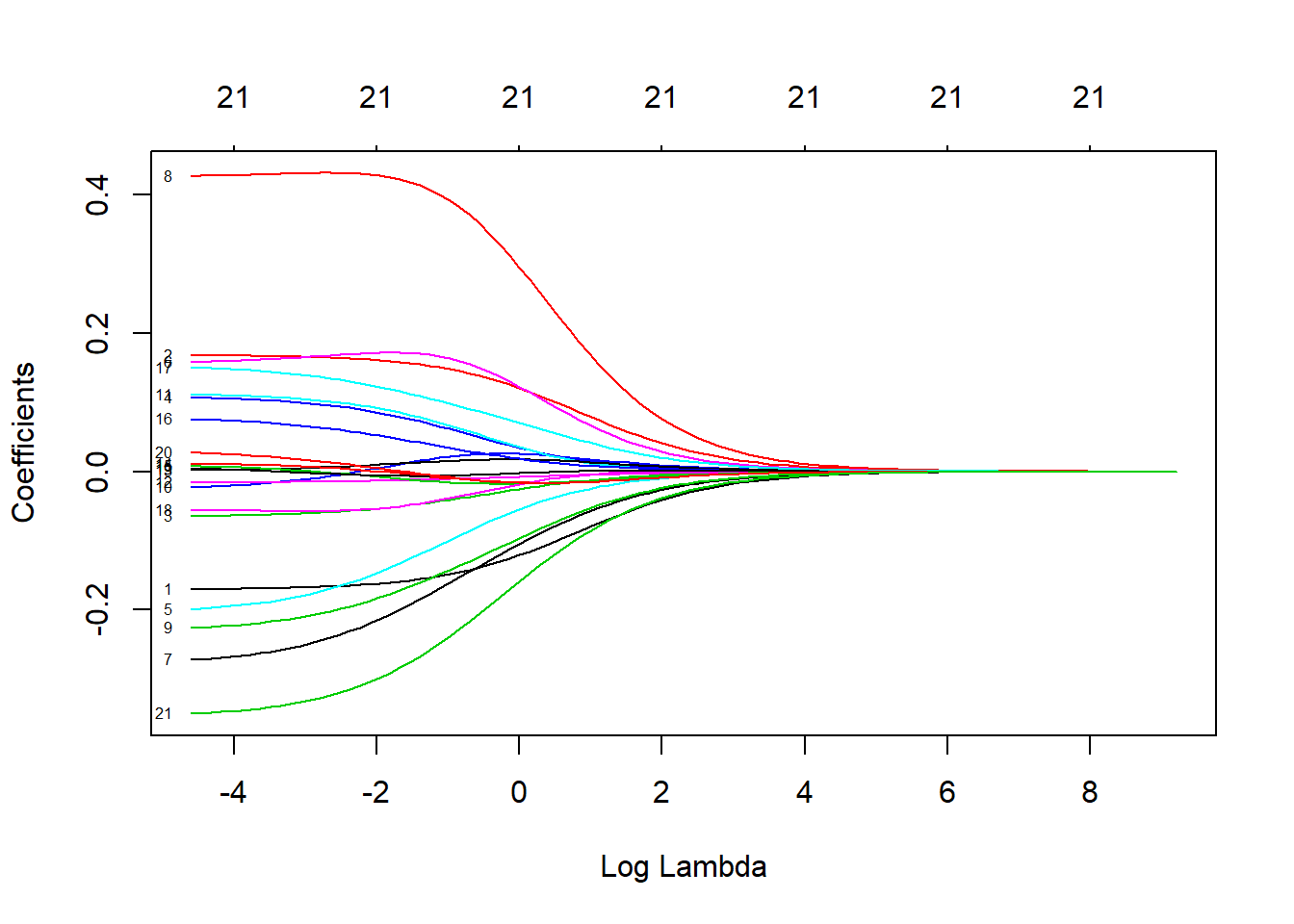
# a set of coefficients for each lambda
dim(coef(ridge.mod))
## [1] 22 100We can look at the coefficients at different values for \(\lambda\). Here, we randomly choose two different values and notice that smaller values of \(\lambda\) result in larger coefficient estimates and vice-versa.
# Lambda and Betas
ridge.mod$lambda[80]
## [1] 0.1629751coef(ridge.mod)[, 80]## (Intercept) RSexMale RSexFemale
## -0.061607390 -0.160606935 0.159900421
## RAge Househld Lab
## -0.051728204 0.082363992 -0.138922683
## SNP Ukip BNP
## 0.172199820 -0.206749980 0.425986910
## GP party.other paper
## -0.176955926 0.008250000 0.088331267
## WWWhourspW religious employMonths
## -0.012922053 0.010790919 -0.001149770
## urbanmore rural urbanmore urban urbanurban
## -0.009100653 0.049660346 0.119249438
## health.goodfair health.goodfairly good health.goodgood
## -0.051779228 -0.006372962 0.002867504
## HHInc
## -0.291172989sqrt( sum(coef(ridge.mod)[-1, 80]^2) )## [1] 0.6911836ridge.mod$lambda[40]## [1] 43.28761coef(ridge.mod)[, 40]## (Intercept) RSexMale RSexFemale
## -0.0024035442 -0.0086089993 0.0086089995
## RAge Househld Lab
## -0.0009024882 0.0009302020 -0.0016851561
## SNP Ukip BNP
## 0.0051999098 -0.0051751362 0.0145257558
## GP party.other paper
## -0.0045065860 0.0018619440 0.0002790212
## WWWhourspW religious employMonths
## -0.0005069474 0.0015920318 -0.0017699007
## urbanmore rural urbanmore urban urbanurban
## -0.0014946533 0.0006218758 0.0040369054
## health.goodfair health.goodfairly good health.goodgood
## 0.0002138639 0.0003043203 -0.0019519248
## HHInc
## -0.0072791705sqrt(sum(coef(ridge.mod)[-1, 40]^2))## [1] 0.02287352We can get ridge regression coefficients for any value of \(\lambda\) using predict.
# compute coefficients at lambda = s
predict(ridge.mod, s = 50, type = "coefficients")[1:22, ]
## (Intercept) RSexMale RSexFemale
## -0.0020916615 -0.0075062040 0.0075062041
## RAge Househld Lab
## -0.0007828438 0.0008050887 -0.0014604733
## SNP Ukip BNP
## 0.0045109868 -0.0045029585 0.0126229971
## GP party.other paper
## -0.0039161618 0.0016221081 0.0002331180
## WWWhourspW religious employMonths
## -0.0004418724 0.0013894830 -0.0015446673
## urbanmore rural urbanmore urban urbanurban
## -0.0013036526 0.0005397837 0.0035149833
## health.goodfair health.goodfairly good health.goodgood
## 0.0001920935 0.0002676711 -0.0017039940
## HHInc
## -0.0063276702Next, we can use cross-validation on ridge regression by first splitting the dataset into training and test subsets.
# cross-validate lambda by splitting dataset into training and test
set.seed(1)
train <- sample(1:nrow(x), nrow(x) * .5)
y.test <- y[-train]
We estimate the parameters with glmnet() over the training set and predict the values on the test set to calculate the validation error.
# fit on training set
ridge.m <- glmnet(x[train, ], y[train], alpha = 0, lambda = grid, thresh = 1e-12)

# predict with lambda = 4
ridge.p <- predict(ridge.m, s = 4, newx = x[-train, ])

# MSE on test data
mean( (ridge.p - y.test)^2 )
## [1] 0.9930511# maximal error?
mean( (mean(y[train]) - y.test)^2)## [1] 1.057127In the previous example, we used \(\lambda=4\) when evaluating the model on the test set. We can use a large value for \(\lambda\) and see the difference in mean error.
# try for large lambda
ridge.p2 <- predict(ridge.m, s = 1e+4, newx = x[-train, ])
mean((ridge.p2 - y.test)^2)
## [1] 1.057087We can also compare the results with a least squares model where \(\lambda = 0\).
# compare to standard logistic regression where lambda is 0
ridge.p <- predict(ridge.m, s = 0, newx = x[-train, ], exact = TRUE)
mean( (ridge.p - y.test)^2 )
## [1] 0.8971826# standard lm
lm.m <- lm(IMMBRIT ~ . -over.estimate -Cons, data = data2, subset = train)
lm.p <- predict(lm.m, newdata = data2[-train,])
mean( (lm.p - y.test)^2 )## [1] 0.897183We can choose different values for \(\lambda\) by running cross-validation on ridge regression using cv.glmnet().
set.seed(1)
# training data for CV to find optimal lambda, but then test data to estimate test error
cv.out <- cv.glmnet(x[train, ], y[train], alpha = 0)
plot(cv.out)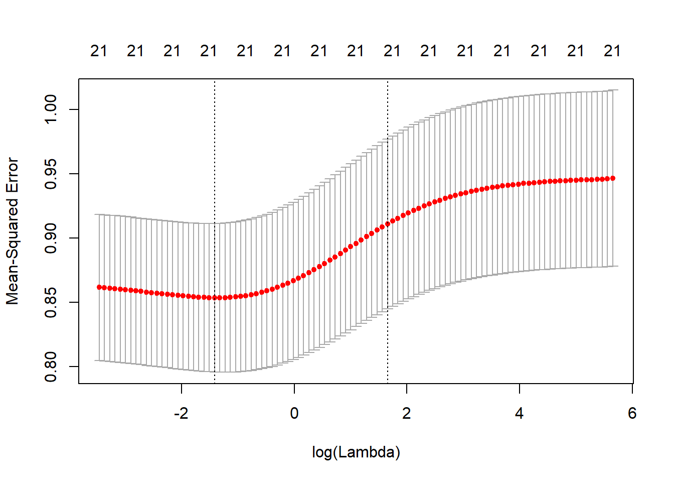
# best performing model's lambda value
bestlam <- cv.out$lambda.min
bestlam
## [1] 0.242911The best performing model is the one with \(\lambda = 0.242911\)
# predict outcomes using best cross-validated lambda
ridge.pred <- predict(ridge.mod, s = bestlam, newx = x[-train, ])
mean((ridge.pred - y.test)^2)
## [1] 0.8635175Finally, we run ridge regression on the full dataset and examine the coefficients for the model with the best MSE.
# ridge on full data
out <- glmnet(x, y, alpha = 0)
predict(out, type = "coefficients", s = bestlam)[1:22, ]
## (Intercept) RSexMale RSexFemale
## -0.059777684 -0.155930812 0.155434688
## RAge Househld Lab
## -0.047003725 0.073306596 -0.120459848
## SNP Ukip BNP
## 0.170611957 -0.185986478 0.414912714
## GP party.other paper
## -0.161476647 0.015342191 0.079032354
## WWWhourspW religious employMonths
## -0.011987748 0.013135994 -0.005108616
## urbanmore rural urbanmore urban urbanurban
## -0.012686943 0.042447233 0.109851218
## health.goodfair health.goodfairly good health.goodgood
## -0.046643963 -0.006836848 -0.002528571
## HHInc
## -0.268558892The Lasso
The lasso model can be estimated in the same way as ridge regression. The alpha = 1 parameter tells glmnet() to run lasso regression instead of ridge regression.
lasso.mod <- glmnet(x[train, ], y[train], alpha = 1, lambda = grid)
plot(lasso.mod)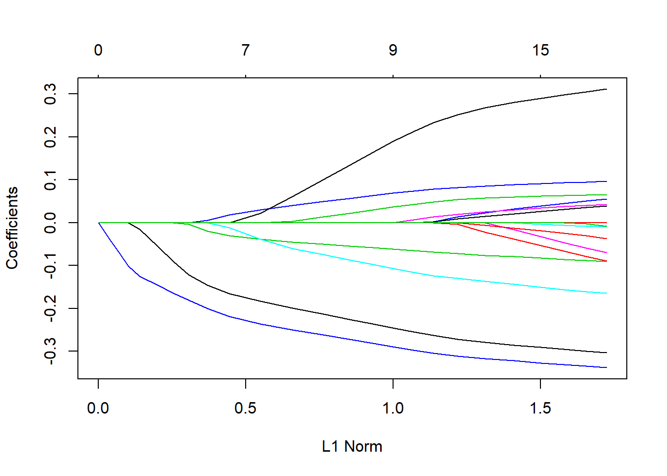
Similarly, we can perform cross-validation using identical step as we did in the last exercise on ridge regression.
# cross-validation to pick lambda
set.seed(1)
cv.out <- cv.glmnet(x[train, ], y[train], alpha = 1)
plot(cv.out)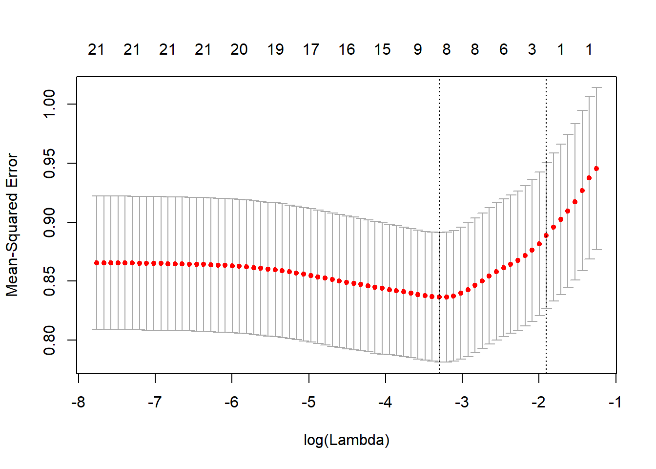
bestlam <- cv.out$lambda.min
lasso.pred <- predict(lasso.mod, s = bestlam, newx = x[-train, ])
mean((lasso.pred - y.test)^2)
## [1] 0.8895347We can compare these results with ridge regression by examining the coefficient estimates.
# compare to ridge regression
out <- glmnet(x, y, alpha = 1, lambda = grid)
lasso.coef <- predict(out, type = "coefficients", s = bestlam)[1:20, ]
lasso.coef
## (Intercept) RSexMale RSexFemale
## 0.124222196 -0.264485052 0.000000000
## RAge Househld Lab
## -0.029577571 0.066394208 -0.070239412
## SNP Ukip BNP
## 0.000000000 -0.029244738 0.261564585
## GP party.other paper
## 0.000000000 0.000000000 0.006077127
## WWWhourspW religious employMonths
## 0.000000000 0.000000000 0.000000000
## urbanmore rural urbanmore urban urbanurban
## 0.000000000 0.000000000 0.021193805
## health.goodfair health.goodfairly good
## 0.000000000 0.000000000lasso.coef[lasso.coef != 0]## (Intercept) RSexMale RAge Househld Lab
## 0.124222196 -0.264485052 -0.029577571 0.066394208 -0.070239412
## Ukip BNP paper urbanurban
## -0.029244738 0.261564585 0.006077127 0.021193805Exercises
Q1
In this exercise, we will predict the number of applications received using the College data set. You need to load libary(ISLR) and then type ?College to get the codebook.
- Split the data set into a training set and a test set.
- Fit a linear model using least squares on the training set, and report the test error obtained.
- Fit a ridge regression model on the training set, with \(\lambda\) chosen by cross-validation. Report the test error obtained.
- Fit a lasso model on the training set, with \(\lambda\) chosen by cross-validation. Report the test error obtained, along with the number of non-zero coefficient estimates.
- Comment on the results obtained. How accurately can we predict the number of college applications received? Is there much difference among the test errors resulting from these five approaches?
Q2
We will now try to predict the per capita crime rate in the Boston data set. The Boston data set is in the MASS library.
- Try out some of the regression methods explored in this chapter, such as best subset selection, the lasso, and ridge regression. Present and discuss results for the approaches that you consider.
- Propose a model (or set of models) that seem to perform well on this data set, and justify your answer. Make sure that you are evaluating model performance using validation set error, cross-validation, or some other reasonable alternative, as opposed to using training error.
- Does your chosen model involve all of the features in the data set? Why or why not?