Solution Day 6 – Regularization
Philipp Broniecki and Lucas Leemann – Machine Learning 1K
Q1
In this exercise, we will predict the number of applications received using the College data set. You need to load libary(ISLR) and then type ?College to get the codebook.
- Split the data set into a training set and a test set.
Load and split the College data.
library(ISLR)
set.seed(11)
sum(is.na(College))
## [1] 0# normalize
College[, -1] <- apply(College[, -1], 2, scale)
train.size <- dim(College)[1] / 2
train <- sample(1:dim(College)[1], train.size)
test <- -train
College.train <- College[train, ]
College.test <- College[test, ]- Fit a linear model using least squares on the training set, and report the test error obtained.
Number of applications is the Apps variable.
lm.fit <-  lm(Apps ~ . , data = College.train)
lm.pred <-  predict(lm.fit, College.test)
mean((College.test[, "Apps"] - lm.pred)^2)
## [1] 0.1027103Test RSS is 0.1027103
- Fit a ridge regression model on the training set, with \(\lambda\) chosen by cross-validation. Report the test error obtained.
Pick \(\lambda\) using College.train and report error on College.test
library(glmnet)
train.mat <-  model.matrix(Apps ~ . -1 , data = College.train)
test.mat <-  model.matrix(Apps ~ . -1, data = College.test)
grid <-  10 ^ seq(4, -2, length = 100)
mod.ridge <-  cv.glmnet(train.mat, College.train[, "Apps"],
                        alpha = 0, lambda = grid, thresh = 1e-12)
lambda.best <-  mod.ridge$lambda.min
lambda.best
## [1] 0.01ridge.pred <- predict(mod.ridge, newx = test.mat, s = lambda.best)
mean((College.test[, "Apps"] - ridge.pred)^2)## [1] 0.1125371- Fit a lasso model on the training set, with \(\lambda\) chosen by cross-validation. Report the test error obtained, along with the number of non-zero coefficient estimates.
Pick \(\lambda\) using College.train and report error on College.test.
mod.lasso <-  cv.glmnet(train.mat, College.train[, "Apps"],
                        alpha = 1, lambda = grid, thresh = 1e-12)
lambda.best <-  mod.lasso$lambda.min
lambda.best
## [1] 0.01lasso.pred <- predict(mod.lasso, newx = test.mat, s = lambda.best)
mean((College.test[, "Apps"] - lasso.pred)^2)## [1] 0.1103055Again, Test RSS is slightly higher than OLS, 0.1027103.
The coefficients look like
mod.lasso <-  glmnet(model.matrix(Apps ~ . -1, data = College),
                     College[, "Apps"], alpha = 1)
predict(mod.lasso, s = lambda.best, type = "coefficients")
## 19 x 1 sparse Matrix of class "dgCMatrix"
## 1
## (Intercept) -2.483323e-02
## PrivateNo 9.101612e-02
## PrivateYes -9.758968e-14
## Accept 8.827830e-01
## Enroll .
## Top10perc 1.285778e-01
## Top25perc .
## F.Undergrad .
## P.Undergrad .
## Outstate -3.693941e-02
## Room.Board 2.682937e-02
## Books .
## Personal .
## PhD -1.307949e-02
## Terminal -1.016626e-02
## S.F.Ratio .
## perc.alumni -1.794075e-03
## Expend 8.228831e-02
## Grad.Rate 1.271356e-02- Comment on the results obtained. How accurately can we predict the number of college applications received? Is there much difference among the test errors resulting from these five approaches?
**Results for OLS, Lasso, Ridge are comparable. Furthermore, it shrinks the Enroll, Top25perc, F.Undergrad, P.Undergrad, Books, Personal, and S.F.Ratio variables to exactly zero and shrinks coefficients of other variables. Here are the test \(R^2\) for all models.
test.avg <-  mean(College.test[, "Apps"])

lm.test.r2 <-  1 - mean((College.test[, "Apps"] - lm.pred)^2) /
  mean((College.test[, "Apps"] - test.avg)^2)

ridge.test.r2 <-  1 - mean((College.test[, "Apps"] - ridge.pred)^2)/
  mean((College.test[, "Apps"] - test.avg)^2)

lasso.test.r2 <-  1 - mean((College.test[, "Apps"] - lasso.pred)^2) /
  mean((College.test[, "Apps"] - test.avg)^2)

barplot(c(lm.test.r2, ridge.test.r2, lasso.test.r2),
        col = "red", names.arg = c("OLS", "Ridge", "Lasso"),
        main = "Test R-squared")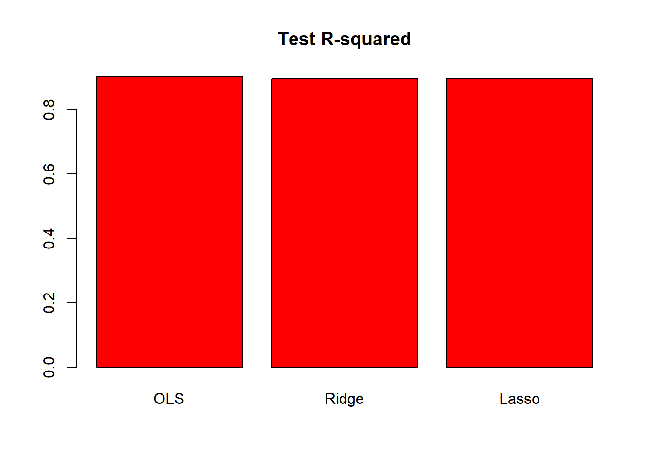
The plot shows that test \(R^2\) for all models are around \(0.9\). All models predict college applications with high accuracy.
Q2
We will now try to predict the per capita crime rate in the Boston data set. The Boston data set is in the MASS library.
- Try out some of the regression methods explored in this chapter, such as best subset selection, the lasso, and ridge regression. Present and discuss results for the approaches that you consider.
set.seed(1)
library(MASS)
library(leaps)
library(glmnet)

# normalize
Boston[, -4] <- apply(Boston[, -4], 2, scale)
Best subset selection
predict.regsubsets <-  function(object, newdata, id, ...) {
    form <-  as.formula(object$call[[2]])
    mat <-  model.matrix(form, newdata)
    coefi <-  coef(object, id = id)
    mat[, names(coefi)] %*% coefi
}

k <-  10
p <-  ncol(Boston)-1
folds <-  sample(rep(1:k, length = nrow(Boston)))
cv.errors <-  matrix(NA, k, p)

for (i in 1:k) {
  best.fit <-  regsubsets(crim ~ . , data = Boston[folds!=i,], nvmax = p)
  for (j in 1:p) {
    pred <-  predict(best.fit, Boston[folds==i, ], id = j)
    cv.errors[i,j] <-  mean((Boston$crim[folds==i] - pred)^2)
  }
}

rmse.cv <-  sqrt(apply(cv.errors, 2, mean))
plot(rmse.cv, pch = 19, type = "b")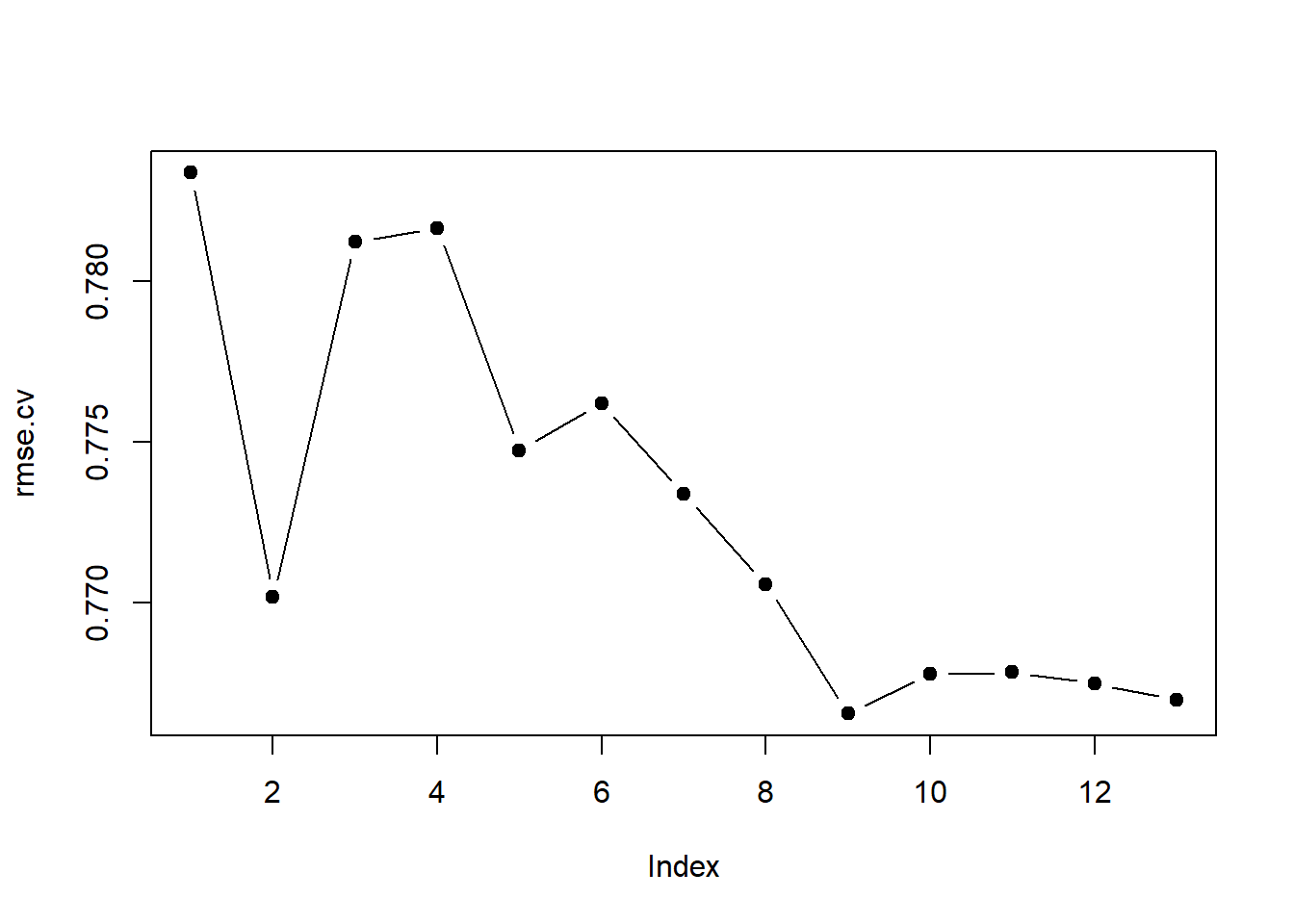
which.min(rmse.cv)## [1] 9rmse.cv[which.min(rmse.cv)]## [1] 0.7665362Lasso
x <-  model.matrix(crim ~ . -1, data = Boston)
y <-  Boston$crim
cv.lasso <-  cv.glmnet(x, y, type.measure = "mse")
plot(cv.lasso)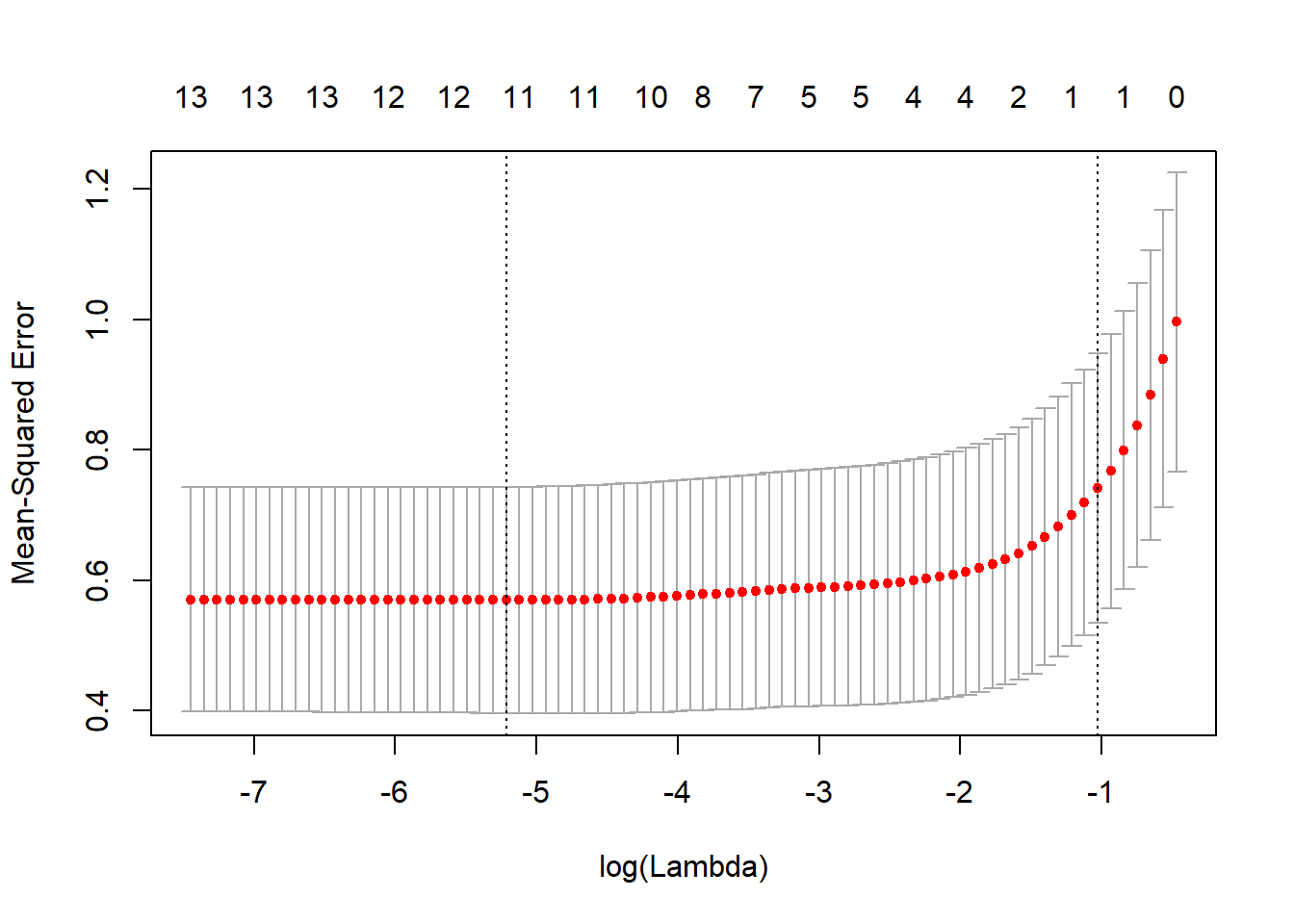
coef(cv.lasso)## 14 x 1 sparse Matrix of class "dgCMatrix"
## 1
## (Intercept) -3.296655e-16
## zn .
## indus .
## chas .
## nox .
## rm .
## age .
## dis .
## rad 2.675681e-01
## tax .
## ptratio .
## black .
## lstat .
## medv .sqrt(cv.lasso$cvm[cv.lasso$lambda == cv.lasso$lambda.1se])## [1] 0.8609123Ridge regression
x <-  model.matrix(crim ~ . -1, data = Boston)
y <-  Boston$crim
cv.ridge <-  cv.glmnet(x, y, type.measure = "mse", alpha = 0)
plot(cv.ridge)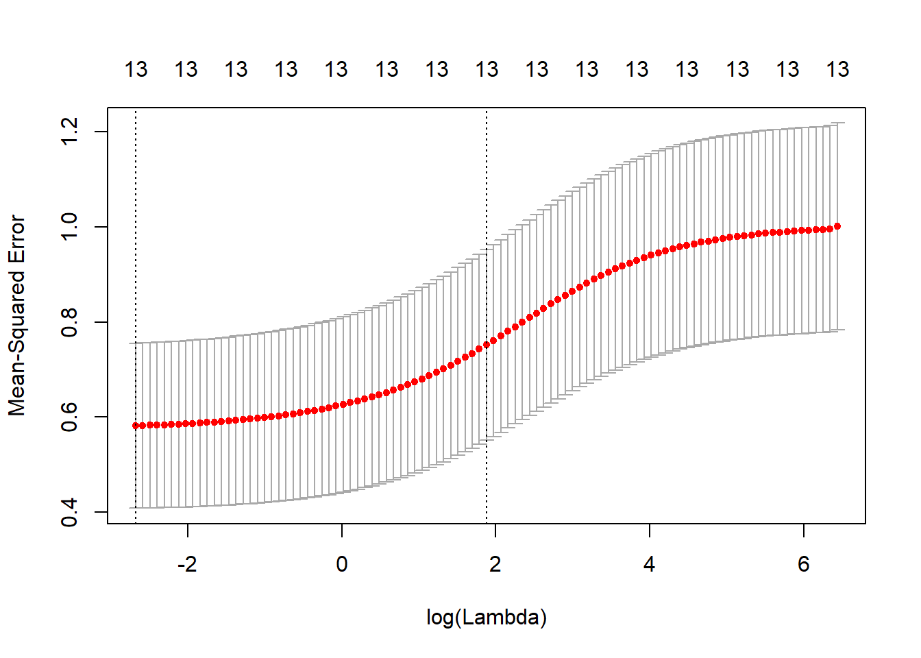
coef(cv.ridge)## 14 x 1 sparse Matrix of class "dgCMatrix"
## 1
## (Intercept) 0.001811369
## zn -0.007607351
## indus 0.027441211
## chas -0.026187226
## nox 0.030309872
## rm -0.013277569
## age 0.024031311
## dis -0.028135246
## rad 0.060548965
## tax 0.052102117
## ptratio 0.021752033
## black -0.035471949
## lstat 0.036940229
## medv -0.031141122sqrt(cv.ridge$cvm[cv.ridge$lambda == cv.ridge$lambda.1se])## [1] 0.866931- Propose a model (or set of models) that seem to perform well on this data set, and justify your answer. Make sure that you are evaluating model performance using validation set error, cross-validation, or some other reasonable alternative, as opposed to using training error.
See above answer for cross-validated mean squared errors of selected models.
- Does your chosen model involve all of the features in the data set? Why or why not?
I would choose the 9 parameter best subset model because it had the best cross-validated RMSE.